


Abstract
We present an analytical model based on the time-dependent WKB approximation to reproduce the photoionization spectra of an H2 molecule in the autoionization region. We explore the nondissociative channel, which is the major contribution after one-photon absorption, and we focus on the features arising in the energy differential spectra due to the interference between the direct and the autoionization pathways. These features depend on both the timescale of the electronic decay of the autoionizing state and the time evolution of the vibrational wavepacket created in this state. With full ab initio calculations and with a one-dimensional approach that only takes into account the nuclear wavepacket associated to the few relevant electronic states we compare the ground state, the autoionizing state, and the background continuum electronic states. Finally, we illustrate how these features transform from molecular-like to atomic-like by increasing the mass of the system, thus making the electronic decay time shorter than the nuclear wavepacket motion associated with the resonant state. In other words, autoionization then occurs faster than the molecular dissociation into neutrals.
Export citation and abstract BibTeX RIS

Content from this work may be used under the terms of the Creative Commons Attribution 3.0 licence. Any further distribution of this work must maintain attribution to the author(s) and the title of the work, journal citation and DOI.
1. Introduction
Fano interference [1] is a ubiquitous feature in the photoionization spectra of atoms. It appears whenever the same continuum state can be reached by direct ionization or through an intermediate doubly excited resonant state with energy above the ionization continuum, which decays via autoionization (AI). The interference of the direct and resonant ionization pathways leads to an asymmetric spectral lineshape, which is well understood and can be used to obtain information on the properties of the resonant state, in particular its energy and AI lifetime.
Analogous resonances exist in molecules [2], where the presence of nuclear motion is of prime importance. In some cases, such as in N2, continuum resonances can be observed in the total ionization cross section, and they have the canonical Fano-type lineshape. In other cases, such as in molecular hydrogen, the lineshapes are very different and can only be seen in the differential cross section.
AI in molecular hydrogen has been extensively studied both theoretically (see, e.g., [2–6]), with an exact numerical solution obtained in [7], and experimentally (see, e.g., [4, 8, 9]). Most experimental studies focused on the dissociative ionization channel, where the formation of the interference patterns can be identified by detecting the H+ fragments. Recently, a theoretical description was proposed that describes the H+ fragment spectral features analytically, using a semiclassical approach [10].
However, the dissociative photoionization channel is by no means dominant in molecular hydrogen. Photoionization leading to the formation of bound  cations is substantially more important. In other molecules, the relative contribution of the dissociative ionization channel is generally even weaker than in H2. This makes the analysis of the resonant features in the photoionization spectra correlated to final bound vibrational states very interesting.
Measurements of vibrationally resolved spectra in molecular hydrogen have recently been performed by means of photoelectron [11] and electron-scattering [12] spectroscopy. Measurements are also available for more complex diatomic and triatomic molecules (see, e.g., [13–16] and references therein). Although the experimental efforts were not aimed at a detailed study of the decay of doubly excited states, the published spectra do show resonant features (which, however, have mostly been ignored so far).
In terms of theoretical approaches, ab initio numerical calculations of vibrationally resolved photoelectron spectra for the non-dissociative channel of molecular hydrogen showed [17] that the spectral features close to the energy of the resonance are very different from the atomic case, supporting the assumption that the nuclear motion should play a profound role in the process. However, to the best of our knowledge, there are no simple models that explain these observations in nondissociative ionization. The key aim of this paper is to develop, both numerically and analytically, a qualitative understanding of the lineshapes appearing in the differential photoionization cross section of molecules. Although the theory is presented for the H2 molecule, for which highly accurate ab initio data is available, it can be extended to any molecular system.
Recently, Ott et al [18] demonstrated how the Fano interference in atoms can be modified in a controllable, time-dependent way by using a second laser pulse, which alters the relative phase between the direct and resonant ionization pathways. Qualitatively, this is also one of the roles played by the coupling between the electronic decay and the nuclear dynamics in molecules: it readily provides the second degree of freedom for influencing the interference between the two ionization pathways. Following resonant excitation, the vibrational dynamics imparts a phase profile on the vibrational wavepacket, which affects the pathways' interference during AI.
Thus, it is not surprising that the AI decay, and the associated lineshape in molecules, is strongly modified or even washed out by the nuclear motion. Its coupling to the electronic decay will be reflected in the final spectra, which will therefore encode the information not only on the electronic but also on the vibrational dynamics. Access to a physically transparent yet quantitative description of the associated process should therefore hold the key to unravelling the coupled electronic and vibrational dynamics.
In atoms, characterization of the Fano lineshapes opened up the possibility of infering properties of resonant states from the photoionization spectra. Here, we develop an analytical description for molecules, which allows one to perform similar analysis for the electronic AI decay strongly coupled to the vibrational motion. Our analytical description is based on a time-dependent semiclassical approach. We first verify its applicability using the example of the Q1 band of doubly excited states of H2 (see figure 1), which converge to the energy of the first  excited state of the
  molecular ion. Subsequently, we use our semiclassical approach to show how the interplay between the timescales of the nuclear motion and the electronic decay determine the final lineshapes obtained in the differential photoelectron spectra.

Figure 1. Illustration of the AI decay of the Q1 doubly excited state of the H2 molecule into the ground state of the  molecule. The decay into bound final states (inset) takes place while the vibrational wavepacket on the Q1 doubly excited state potential energy surface is still in the vicinity of the inner classical turning point. Later decay leads to a dissociating wavepacket.
Download figure:
Standard image High-resolution imageThe article is structured as follows. Section 2 introduces numerical and analytical methods used to simulate and interpret the signatures of the AI decay in molecules. Section 3 presents the results and demonstrates that the vibrationally resolved measurements of the AI spectra can be reproduced using simplified numerical calculations. Finally, section 4 contains a discussion on the formation of the molecular AI lines for low vibrational bound states, the role of the nuclear motion, and the transition to the atomic limit.
2. Methodology
In this work, we develop an analytical approach to describe the AI decay in molecules and compare it with the solution of a full dimensional calculation solving the time-dependent Schrödinger equation (TDSE) for the H2 molecule.
To evaluate the accuracy of the analytical model presented in this work, we use as reference data the energy spectra obtained in the TDSE calculation, where the time-dependent wave function is expanded in a basis set of Born–Oppenheimer (BO) eigenstates of the isolated molecule, which are products of H2 electronic and vibrational states. Because we are using the eigenstates, the ionization amplitudes are directly given by the time-dependent coefficients of the expansion as long as the asymptotic limit is reached. In this approach, the molecular structure is computed using a Feshbach-like method that projects the total Hamiltonian in two separated half-spaces (P and Q). The subspaces are built such that, in the single ionization continuum, the Q subspace will hold the doubly excited states, while the P subspace holds the background continua. This approach allows an intuitive analysis of the AI decay from the Q states into the P states. A detailed description of the method is given elsewhere [19–21], and therefore we will not describe it here.
Alongside the TDSE calculation, we introduce a truncated calculation, referred to here as the 'three-state model', which uses a minimal basis set essential to describe the AI decay. It reduces the basis to a single electronic BO curve for the initial, intermediate, and final states and a single electronic continuum correlated to the ground electronic state of  . We then numerically solve the TDSE within this restricted basis of electronic states (i.e., it is a hybrid representation where the vibrational wavepacket is propagated on a coordinate grid, while the electronic continuum is expanded in the spectral basis). This method is described in section 2.1.
Finally, we derive our analytical approximation, the semiclassical method, and use it to calculate the vibrational wavepacket dynamics associated with the intermediate doubly excited electronic state prior to decay. Its results allow us to describe the final spectra while keeping a clear physical connection to the classical trajectories that guide the wavepacket. The method is described in section 2.2.
2.1. Three-state model
We start by introducing the following ansatz for the wavefunction:

where  and
and  are electronic wavefunctions for the ground and doubly excited state of H2, respectively. The latter is the intermediate state that decays, due to AI, into the ground state of the
  molecule.
  is the final state wavefunction representing one electron with momenta
  in the continuum, plus a bound electron;
  are the corresponding vibrational wavepackets. The TDSE then reads (atomic units are used everywhere)

where  is the nuclear kinetic energy,
  includes the electronic kinetic energy and the electron-nuclear interaction,
  is the electron-electron interaction, and
  is the interaction with the electromagnetic field. The latter can be expressed as
  , where
  is the dipole operator and
  is the laser electric field.
Applying the adiabatic approximation, we obtain three coupled equations:


where the dependence on R is implicit for all functions except  . Vg and Va are the ground and Q1 BO potentials of the H2 molecule and Vion is the
  ground state BO potential of the
  molecular ion.
  are the dipole couplings between different electronic states and
  is the electron-electron coupling between the autoionizing state and the electronic continuum state.
This three-state model is very similar to the full ab initio calculation. Approximations are made by keeping a single ionization channel (l = 1) and using the adiabatic approximation, which neglects non-BO effects during the nuclear motion along the Q1 state. The model excludes first excited  and all other higher-energy states of the dihydrogen ion. On the other hand, the exact electrostatic couplings between the electronic states extracted from the ab initio method are used. Finally, the Q1 series of doubly excited states of the H2 molecule consists of many closely spaced doubly excited states. Here it is limited to a single lowest-energy state that has the largest ionization cross section.
The final vibrational population and the photoelectron spectra can be extracted from  . Note that the
  part is calculated for every continuum state, leading to a mixed spectral-grid representation of the photoelectron-vibrational wavefunction.
2.2. Analytical model
To treat the problem analytically, we first simplify equations (3a )–(3c ) by adiabatically eliminating the continuum from equation (3b ) for the wavepacket in the bound Q1 part of the autoionizing state. This approximation is known to give adequate results when applied to the AI of H2 (see, e.g., [2–4, 22] for a detailed discussion). By introducing the decay width

we can rewrite equations (3b ) and (3c ) as:


where the dependence on R is again implicit. The above set of equations implies that the Q1 state BO potential acquires a complex component,  .
.
2.2.1. Analytical solution for a vibrational wavepacket on the intermediate state
First, we neglect the decay of the vibrational wavepacket propagating along the  potential energy curve (PEC) of the Q1 state and write it as

where  normalizes the wavepacket to unity. A Gaussian wavepacket is a good approximation for the ground vibrational state of most molecules. Moreover, the shape of the wavepacket will be preserved after excitation by a short laser pulse in the sudden excitation limit.
We now substitute the ansatz into the TDSE for the vibrational motion along the  potential. This leads to the Hamilton-Jacobi equation for the phase
  :
:

where μ is the reduced mass of the nuclei and, as usual for the WKB method, the second-order derivative of  is neglected. Let
  be the classical trajectory that starts at the center of the initial wavepacket with zero initial momentum and moves along the potential,
  following the usual Newtonʼs equations. We now expand the
  PEC in a Taylor series up to the second order around this classical trajectory,
  :
:

Accordingly, we look for a solution for  in a polynomial form, up to the second order in powers of Rcl:

Here the momentum,  is conjugated to the coordinate
  and corresponds to the solution of Newtonʼs equations of motion on the potential energy surface,
  . The action,
  is the classical action accumulated along the trajectory
  and
and  is the time-dependent width of the wavepacket. The above polynomial expansion implies that the initially Gaussian wavepacket, created by photo absorption into the Q1 state, maintains its approximately Gaussian shape while acquiring a time- and R-dependent phase profile. This approximation proved quite accurate, especially during the initial stage of propagation. For H2, this corresponds to times
  which we found to be sufficient for the AI decay into the bound vibrational states to occur.
Using equations (7)–(9) and leads to the following expression for the time-dependent wavepacket:

where  is
is

expressed via the parameter C

and the curvature of the potential,  (i.e., the second derivative of the potential at
  ). Finally, X0 is a parameter related to the initial width of the wavepacket:

In the presence of AI decay,  acquires a complex component,
  . Including it in the 0-th order into equation (8) introduces an additional term

2.2.2. Interference of direct and resonant ionization channels
Upon photoionization, the population of a particular final vibrational state, ν, correlated to the photoelectron with energy  can be written as a coherent superposition of the direct (
 ) and AI (
 ) contributions:

where the direct contribution is calculated as

and the AI contribution as

Here,  is the ν-th vibrational eigenstate of the
  ground state potential curve of
  with a total vibronic (electronic and vibrational) energy, Ev.
  is the vibrational wavepacket on the PEC of the Q1 state, which we evaluate using equation (14).
  accounts for the spectral components of the short laser pulse

where  is the laser electric field and
  is the detuning between the initial vibronic state Eg, the final vibronic continuum state
  and the carrier frequency ω

2.3. Computational details
The time propagation of the vibrational wavepacket associated to the coupled PECs described by equations (3a
)–(3c
) was performed in the length gauge using a Cranck-Nicholson scheme. Some of the parameters used in the calculation are summarized in table 1. The maximum propagation time, 4 fs, ensures that the asymptotic limit is reached for both dissociative and non-dissociative ionization components. The H2 ground state potential was obtained from [23] and used to calculate the initial vibrational wavepacket,  by solving the one-dimensional vibrational eigenvalue problem in a B-spline basis set. We use as discretized electronic continua a set of potential energy curves that are parallel and equidistant in electron momentum with respect to the ground state of
  . The former has been accurately calculated using Powerʼs one-electron diatomic molecule code [24, 25]. The potentials
  and electronic couplings between the electronic states at different values of R are extracted from the ab initio calculations [19, 21].
Table 1. Summary of parameters used in the calculations.
| propagation time, tmax | 4 fs |
| time step, Δt | 3/4 as |
| internuclear distance grid length, R | 25 au |
| internuclear distance grid spacing, dR | 0.01 au |
| number of continuum states, N | 99 |
maximum continum energy, 
|
53 eV |
| H2 reduced mass, μ | 918.58 au |
| H2 equilibrium internuclear distance, R0 | 1.4325 au |
| initial width, X0 | 0.2364 au |
The analytical solution from our model, as described in section 2.2, was evaluated by first calculating a classical trajectory along the  surface starting at the H2 equilibrium internuclear distance, R0, to obtain
  ,
,  and
and  . They were then used in equations (10)–(13) to evaluate
  and subsequently
  . The decay width,
  was extracted from the full electrostatic couplings,
  as described in [3].
The vibrational eigenvalues,  and vibronic energies, Ev, were calculated using
  PEC. The integrals over R and t in equations (16) and (17) were performed numerically, where the
  and dipole couplings between PECs were the same as in the three-state model calculation.
Finally, the ionization probabilities were normalized to the bandwidth of the laser pulse unless stated otherwise. This was done by dividing the probability of the final state with energy, , by the amplitude of the laser pulse spectra at the frequency, , as described in [26].
3. Results
The vibrationally resolved photoionization probabilities obtained from the full and truncated calculations, as introduced in section 2, are plotted in figure 2 and compared with results from the semiclassical model. The calculations were carried out with a single attosecond extreme-ultraviolet (XUV) pulse. The pulse had a duration of 400 as (appreciably shorter than the autoionization lifetimes for H2 [10, 17]) and a central photon energy of 30 eV, which in resonance with the first doubly excited state of the Q1 series. The laser intensity was set to I = 109 W/cm2, which is low enough to ensure a perturbative regime. This gives a direct correspondence between the total cross sections and ionization probability for any photon energy within the bandwidth of our pulse [26].

Figure 2. Vibrationally resolved photoionization probability demonstrating the traces for AI decay calculated using (a) ab initio numerical method, (b) the reduced three-state model, and (c) and the analytical treatment.
Download figure:
Standard image High-resolution imageThe transition probabilities obtained using the ab initio approach are presented in figure 2(a). They match the equivalent results obtained using the time-independent approach reported in [17]. The effect of the resonance can be clearly seen as a modulation of the transition probability, which spans a much broader photon energy range and has a smaller amplitude than those found in the atomic ionization cross section close to a resonance (see, e.g., [27]). Note, however, that due to a systematic shift of the modulation pattern in photoelectron energy for different νʼs, no resonance traces would be observed for vibrationally unresolved spectra. In general, the full atomic photoionization probability and the differential molecular probabilities presented here are qualitatively very different. The origin of these differences will be the focus of section 4 of this paper.
The results obtained using the 'three-state model' (figure 2(b)) are in excellent agreement with the ab initio reference results. This shows that a reduced dimensionality model calculation for the time-dependent dynamics allows us to quantitatively reproduce the results of a more sophisticated ab initio TDSE calculation. Of course, this implies that the same electrostatic dipole matrix elements are used in both cases. Importantly, it shows that the AI dynamics in the H2 molecule at this energy range can be successfully described by the three PECs, validating the three-state truncation used en route to deriving the analytical model (see section 2.2).
Good agreement between the 'three-state model' and the ab initio calculation shows that it is possible to simplify the analysis of correlated electron-nuclear dynamics by performing time-dependent propagation for relevant coupled potential energy surfaces. This is important for more complex molecules, where the evaluation of the exact coupling-matrix elements may not be feasible. However, it will still be possible to use reduced-dimensionality TDSE calculations and infer the correct coupling elements by comparing them with experimental data.
The probabilities obtained using the analytical approach are shown in figure 2(c). They are in good agreement with both the ab initio and the three-state model results. The exact details, such as the exact positions of minima and maxima for different vibrational states, differ slightly compared to those of the more sophisticated models. In particular, the analytical calculation overestimates the modulation of the ionization probabilities close to the resonance. However, considering the simplicity of the approach, the qualitative agreement is excellent and captures all relevant physical effects governing the AI dynamics in the H2 molecule.
The effects of the interference between the direct and resonant ionization channels become clearer upon inspecting the final ionization probability as a function of both the vibrational state and the photoelectron energy. Such spectra, presented in figure 3, allow one to more easily identify the key spectral features and the correlations between different vibrational states. Note that unlike the previous data, the spectra in figure 3 are not divided by the laser spectral density, and therefore depend on the laser pulse parameters.

Figure 3. Differential photoionization probabilities (differential in vibrational and photoelectron energies) for a 400 as pulse centerd around 30 eV photon energy obtained using (a) ab initio, (b) reduced three-state, and (c) analytical approaches. The probability distribution of the direct-only channel, which is indistinguishable for different models, is plotted in (d). The difference between the (a) ab initio and (d) direct-only probabilities is plotted in (e). (f) shows the same difference spectra for the analytical calculation. Plots (e) and (f) have a shifted color scale to accommodate negative (blue) and positive (red) values. Note that the discontinuities in the plotted probability distribution arise because discrete spectra of bound vibrational states are represented on the horizontal axis.
Download figure:
Standard image High-resolution imageA comparison of the results obtained using different methods shows a similar trend to that seen in figure 2. The three-state calculations are in excellent agreement with the ab initio results, while the analytical spectra provide a qualitatively similar picture, correctly capturing all spectral features, but overestimating the modulations.
The effect of the interference between the direct, and the AI pathways is revealed most clearly by looking at the difference spectra obtained with and without including the AI decay, as seen in figures 3(e) and (f). The interference pattern resembling a Fano profile can be identified although, as it will be clear later, its origin is very different. A minimum due to destructive interference can be seen for photoelectron energies between 10–15 eV, while a maximum due to constructive interference appears around 8–10 eV. For each individual vibrational state, the maximum is shifted to lower photoelectron energies compared to the 'direct only' channel. Finally, the interference minima and maxima for higher vibrational energies shift to higher photoelectron energies, creating a tilted shape of the overall spectra. These features are present in the ab initio results (figure 3(e)), the three-state model (not shown), and in the analytical calculation (figure 3(f)).
To summarize, the semiclassical analytical model of molecular photoionization in the presence of a continuum resonance proved capable of reproducing all essential qualitative features of the full spectrum, resolved both on the photoelectron energy and the vibrational eigenstate of the cation. The model works for steep potentials in good agreement with previous, more standard WKB methods. Moreover, it also yields no difficulties when starting the wavepacket motion at the turning point of the classical trajectory (where application of standard WKB methods requires extra care), and works well for describing transitions to the bound vibrational states on the  surface with high
  (the semiclassical region) and the states with low
  (the quantum region). In the following section, this analytical model will be used to explain the origin of the observed spectral features.
4. Discussion
The disappearance of Fano-like interferences in the AI decay of the H2 molecule was previously discussed and modelled by Palacios et al [10] for the dissociative spectra of H+ fragments. It was shown that the interference patterns are dominated by the phase difference accumulated by the vibrational wavepackets propagating along the direct channel (the  surface) and the AI dissociation channels (the Q1 surface) up to a transition point Ri, masking the atomic-like Fano interference.
The method used in [10] is based on the time-independent WKB approach and is not suitable for the nondissociative channel. Its direct application meets with technical difficulties when applying it to the dynamics involving low vibrational states, especially in the vicinity of the classical turning points of the potential. In particular, in the semiclassical treatment [5, 6, 10], the transition from the AI state potential curve to the  curve takes place at the point, Ri of the classical trajectory where the classical momenta associated with vibrational motion on the two potential curves become equal. In other words, both energy and momentum at the transition point are conserved. In contrast to the dissociative vibrational continuum, bound vibrational state carry low momentum and should therefore be populated while the vibrational wavepacket on the AI surface is still close to the classical turning point, where the time-independent WKB method is not applicable. Moreover, for the lowest vibrational states the condition of equal momenta at the transition point Ri is never satisfied for any real value of Ri.
To illustrate this point further, we examine the time dependence of the AI decay into final vibrational states with low (ν = 0) and high (ν = 10) quantum numbers. These represent respectively 'quantum' and 'semiclassical' final states. The transition probability is obtained by evaluating the time-dependent dipole matrix element,  between the Q1 and
  states used in the equation (17). Its value as a function of time for the two different final vibrational bound states is plotted in figure 4(a). We can clearly see that while the transition probability into the ν = 10 final vibrational state is peaked at a certain time, the equivalent probability into the ν = 0 final state decreases monotonically with time, and is therefore not clearly associated with a specific transition point, Ri.
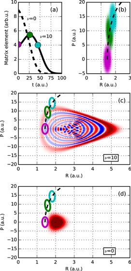
Figure 4. (a) The Franck-Condon (FC) overlap of the vibrational wavepacket on the Q1 state with the ν = 0 and ν = 10 final bound vibrational states of the 
 state potential as a function of time. (b) The Wigner representation of the vibrational wavepacket on the Q1 surface at three different times marked in (a), where the dashed line shows the classical trajectory. The same data is represented in (c) and (d) as contour lines, where they are overlapped with the phase-space representation of the (c) ν = 10 and (d) ν = 0 vibrational state distributions.
Download figure:
Standard image High-resolution imageThe difference between the curves in figure 4(a) can be understood from the dynamics of the vibrational wavepacket on the  surface in the Wigner phase space representation. It is shown in figure 4(b) for three values of time: before, after, and at the most likely AI decay time for the ν = 10 final state. During this time the wavepacket does not move significantly along the position coordinate, R. However, its evolution along the momentum axis is substantial. Hence, the time dependence of the AI decay probability into a specific bound vibrational state is determined not by the motion of a vibrational wavepacket on the intermediate state potential, but by the much more rapid evolution of its momentum. We can conclude that a momentum 'kick' that the wavepacket receives when it is created on a steep potential curve creates a phase mask that determines the overlap with the final vibrational bound state it decays into.
The time evolution of the transition probability can be better understood by examining the phase space distributions of the vibrational wavepacket on the  curve with the final bound state eigenfunction
  as shown in figures 4(c) and (d). Note that the overlap between two wavefunctions in the Wigner representation can be expressed as
  . For ν = 10, the maximum in the transition probability is reached when the vibrational wavepacket on the
  curve leaves the region where the ν = 10 state is highly oscillatory and reaches its edge, which is relatively smooth. For the ν = 0 vibrational state, on the other hand, the wavepacket on
  surface starts away from the maxima of the final state distribution and never crosses it. As a result, the AI decay probability into this state decays monotonically with time. This is why no clear 'classical' transition point, Ri, can be defined. We note again that in both the ν = 0 and ν = 10 cases, the evolution predominantly takes place along the momentum and not along the position axis.
An intuitive way to understand the connection between the shape of spectral lines and the dipole response function in a time domain picture was presented by Ott et al [18], who demonstrated that a short laser pulse can give a 'kick' to the time-dependent dipole response of an atomic system, which introduces an additional phase shift. The latter translates into the modification of the Fano spectral lineshape. In molecules, this 'kick' is provided naturally due to the momentum evolution of the vibrational motion. However, in this case it leads not to a single phase shift, but to a phase profile across the vibrational wavepacket, which determines the appearance of the spectral lines.
We now focus our attention on the difference between the atomic and molecular spectra at resonance. For atoms, the lineshape corresponds to the well-known Fano profile [1]. We will now analyze how the shape of the vibrationally resolved molecular photoionization spectra is modified by the interplay between the electronic decay, characterized by the  width, and the nuclear motion. Specifically, we shall look at the spectral lineshapes defined as the ratio between the full ionization probability and the probability associated with the direct channel only,
  . This allows us to deconvolve the spectra from the laser pulse parameters and the cross section of direct ionization, and focus on the effect of the interference between the direct and resonant contributions.
To examine the role of the nuclear motion, we begin by gradually increasing the reduced mass of the nuclei while simultaneously leaving the electronic system intact. This corresponds to dihydrogen isotopes, deuterium and tritium, as well as to fictitious systems with heavier nuclei. The lineshapes for different masses are plotted in figure 5. As the mass is gradually increased, the lineshapes get narrower and deeper while the position of minima and maxima shift towards higher energies. The infinite mass limit obtained in our calculation agrees well with the ab initio calculations performed for the hydrogen molecule in the fixed nuclei approximation in [27] (see the inset of figure 5).

Figure 5. The dependence of the lineshape on the reduced mass of the nuclei for masses that are 1, 2, 20, and 100 times bigger than the mass of H2. The lineshapes correspond to the ν = 2 vibrational eigenstate. The inset shows a comparison between the ionization cross section obtained from the TDSE calculation, where the mass of the nuclei was increased by a factor of 100 (red line), and the ab initio results in the fixed nuclei approximation obtained from [27] (black line).
Download figure:
Standard image High-resolution imageThe transformation of the spectra in figure 5 can be understood by analyzing the time dependence of the transition probability for different masses. Approximating the decay width with its value at the equilibrium internuclear distance,  we can rewrite the transition dipole as

Hence, the AI transition probability is determined by two timescales. The first is due to the electronic decay governed by the term  . It yields an exponential decay of the resonant state population, exactly as in the atomic case. The vibrational dynamics of a molecule leads to the second timescale due to the time-dependent Franck-Condon (FC) overlap,
  between the wavepacket in the resonant state and the final vibrational eigenstate.
The interplay between these two timescales for different masses of the system is illustrated in figure 6. For small masses and hence rapid nuclear evolution, which is the case for the H2 molecule, the decay of the FC overlap is much faster than the electronic decay determined by  . As a result, the time dependence of the transition probability into a particular final vibrational state, ν, is governed by the FC overlap; once the wavepacket on the
  curve starts moving and the FC overlap decays, the transition probability vanishes. Importantly, the FC overlap into a particular vibrational state vanishes much faster than the time the nuclei take to move any appreciable distance (see figure 4).

Figure 6. FC overlap time dependence for ν = 2 with (solid lines) and without (dotted lines) electronic decay  for different nuclear masses. The black solid curve shows purely electronic decay without nuclear motion.
Download figure:
Standard image High-resolution image
Thus, for light molecules the observed lineshapes are governed by the nuclear motion. As the mass increases, the vibrational dynamics slows down and the FC time window increases. As it becomes longer, the electronic decay due to  acquires a larger influence on the overall time dependence of the decay. For a mass 100 times bigger than the original mass of H2, the AI decay probability is dominated by the timescale of the electronic decay, and the vibrationally resolved lineshape starts resembling the atomic case. Also note that the decay probability as a function of time transforms from a non exponential decay for a small mass to a pure exponential decay for a big mass. In systems other than the H2 molecule, where the nuclear motion is extremely fast (or the decay is slow), we expect the two timescales to be comparable and hence to play equal roles in the formation of the photoionization spectra.
5. Conclusions
We have demonstrated an analytical approach that can describe the decay of autoionizing states into the final bound vibrational eigenstates of molecules. The method is based on the time-dependent semiclassical approximation, and it accurately describes vibrational dynamics in the regions of the potential energy surfaces where quantum effects are strong and the time-independent semiclassical approximations encounter difficulties. Comparison with ab initio calculations for the hydrogen molecule shows that our model provides a faithful description of the underlying dynamics.
Using the developed methodology, we showed that the lineshapes arising in vibrationally resolved one-photon ionization of molecular hydrogen close to the energy of the Q1 resonance are very sensitive to nuclear dynamics in the resonant state. Importantly, it is not the motion along the internuclear coordinate of the wavepacket, but the chirp it acquires due to the momentum 'kick' on the dissociating surface that is the determining factor in the formation of the spectrum. Finally, we showed how the final spectral lineshape can change from molecular-like to atomic-like with increasing molecular mass because of the interplay between timescales arising due to the nuclear motion, through the FC overlap, and due to the electronic decay, through the decay width, Γ.
The maxima of the FC overlap of the resonant state with different final vibrational states is obtained at different times after the ionization. As a result, the lineshape correlated with each individual vibrational state reflects a snapshot of the dynamics on the resonant state during a certain time window. This can be viewed as a 'molecular clock' and could, in principle, be used to recover the vibrational dynamics on the resonant state potential and/or the lifetime of AI decay. This possibility will be explored in a later work.
This work uses the H2 molecule as a reference system because highly accurate ab initio calculations, potential energy surfaces, and dipole coupling are available, allowing one to test the validity of our methodology. Nevertheless, it can be used as a 'recipe' to study other molecular systems. Moreover, the description is not limited to doubly excited electronic states embedded into the ionization continuum, but could in principle be applied to any transient state that decays by emitting an electron. For example, the resonant Auger decay, where nuclear motion in the core excited states has a strong influence on the final Auger electron spectra, can be a possible target of study (see [28, 29] and the references therein).
Finally, the atomic Fano resonances have recently become an active field of study in the ultrafast physics community, with direct time-dependent spectroscopic approaches used to trace the decay of resonant states [30, 31]. The prime goal of these experiments was to test and refine the tools of ultrafast pump-probe spectroscopy for studying correlated electronic dynamics. Doubly excited states of atoms provided an excellent test bed for such studies. The analysis of coupled electronic and nuclear dynamics on the 1-fs time-scale in molecules appears to be a natural and interesting extension of such experiments. We believe that the time-dependent approach developed here will provide a recipe to interpret ultrafast time-resolved experiments in molecular systems.
Acknowledgments
We acknowledge computer time from the CCC-UAM and Mare Nostrum supercomputer centers and financial support by the European Research Council under the ERC Advanced Grant no. 290853 XCHEM, FP7 Marie Curie ITN CORINF, FP7 Marie Curie IRG ATTOTREND, the Ministerio de Economa y Competitividad projects FIS2010-15127, FIS2013-42002 R and ERA-Chemistry PIM2010EEC-00751, the European COST Action CM1204 XLIC, and EPSRC programme no. EP/I032517/1.