


Abstract
In recent years, the gap between theory and practice in quantum key distribution (QKD) has been significantly narrowed, particularly for QKD systems with arbitrarily flawed optical receivers. The status for QKD systems with imperfect light sources is however less satisfactory, in the sense that the resulting secure key rates are often overly dependent on the quality of state preparation. This is especially the case when the channel loss is high. Very recently, to overcome this limitation, Tamaki et al proposed a QKD protocol based on the so-called 'rejected data analysis', and showed that its security—in the limit of infinitely long keys—is almost independent of any encoding flaw in the qubit space, being this protocol compatible with the decoy state method. Here, as a step towards practical QKD, we show that a similar conclusion is reached in the finite-key regime, even when the intensity of the light source is unstable. More concretely, we derive security bounds for a wide class of realistic light sources and show that the bounds are also efficient in the presence of high channel loss. Our results strongly suggest the feasibility of long distance provably secure communication with imperfect light sources.

Content from this work may be used under the terms of the Creative Commons Attribution 3.0 licence. Any further distribution of this work must maintain attribution to the author(s) and the title of the work, journal citation and DOI.
1. Introduction
The gist of quantum key distribution (QKD) [1–3] is that it allows two remote parties, Alice and Bob, to establish common secret keys in the presence of an adversary, Eve, who may have unlimited computing resources and technological advances. Today, three decades after its introduction, QKD has made enormous progress in both theory and practice, and is arguably on the verge of global commercialization. Having said that, however, there are still some issues, both theoretical and experimental, that need to be resolved before we can reach that level. Amongst those, the most pressing one is the mismatch between device models used in security proofs and actual devices used in QKD systems. In particular, such implementation loopholes can lead to side-channel attacks that break the security of QKD. Notably, it has been repeatedly demonstrated that the behaviour of single-photon detectors employed in QKD systems can be externally controlled, simply by exploiting their physics [4]. In this case, it is easy to verify that security cannot be achieved, since the measured data are not representative of the quantum channel [5]. Undoubtedly, such hacking demonstrations raise not only the importance of proper calibration of QKD systems, but also the importance in developing security proof techniques that can tackle modeling discrepancies. Indeed, in the past few years, much attention has been devoted towards the development of such proof techniques and side-channel countermeasures, particularly in the areas of security of finite-length keys [6–10] and detector side-channel attacks [11, 14, 15, 12, 13].
Amongst these theoretical results, only a few considered the issue of state preparation flaws—despite that it is a commonly faced experimental problem. More concretely, typical light sources used in QKD systems are not true single-photon sources and practical optical modulators employed to encode the light pulses are inherently limited in precision. The former can be resolved by using the decoy-state method [16–18], which allows QKD systems based on practical light sources to achieve the security performance of single-photon QKD. The latter, however, does not have an adequate solution. In particular, it has been firstly shown by Gottesman et al [19] that such inaccuracies in encoding can lead to very pessimistic secret key rates in the presence of high quantum channel loss. Also, other works show similar results [20]. This strong dependency on channel loss is primarily due to the fact that state preparation flaws can be seen as a form of basis information leakage, which gives Eve some advantage in formulating basis-dependent attacks. Crucially, as shown in [19, 20], Eve's advantage can be significantly enhanced by exploiting channel losses. Consequently, this heavily penalizes the secret key rate whenever the channel loss is substantial.
Very recently, a loss-tolerant QKD protocol [21] has been proposed by Tamaki et al as a means to overcome typical encoding flaws in QKD systems. More specifically, as briefly mentioned earlier, here we are considering encoding flaws due to imprecise alignment of optical modulators. For example, if the quantum states are encoded into the polarization degree-of-freedom of photons, an encoding flaw could be due to a misalignment in the wave-plate used to set the desired polarization. The protocol is similar to the Bennett–Brassard 1984 (BB84) QKD scheme [22], but instead of considering all the four BB84 states, it uses only three of them. Interestingly, by considering statistics beyond those of the BB84 protocol, the resulting secret key rate is the same as the one of BB84's [23–27]. More importantly, the secret key rate has the very nice property in that it is almost independent of encoding flaws. These results imply that the usual stringent demand on precise state preparation can be considerably relaxed and one only needs to know the prepared states. Additionally, it is useful to mention that most current BB84 QKD systems can easily switch to the loss-tolerant QKD protocol without much hardware modifications.
In anticipation that the loss-tolerant QKD protocol will be widely implemented in the near future, we extend the security analysis in [21] to the finite-key regime, i.e., we derive explicit bounds on the extractable secret key length (in [28], the authors have implemented the loss-tolerant protocol experimentally with careful verification of the qubit assumption used in the protocol. This paper also includes some finite-key analysis of the protocol. Unfortunately, however, its phase error rate estimation seems to be valid only against collective attacks). Furthermore, our bounds can be applied to a wide range of imperfect light sources —including typical cases whereby the intensity of the laser is fluctuating between a certain range6 .
Also, the security bounds are obtained within the so-called universal-composable framework [30], and thus secret keys generated using these bounds can be applied to other cryptographic tasks like the one-time-pad. In order to investigate the feasibility of our results, we consider a QKD system model that borrows parameters from recent fibre-based QKD experiments. With this realistic model, our numerical simulations show that provably-secure keys can be distributed up to a fibre length of about 120 km, even when only 1011 signals are sent by Alice to Bob.
This paper is organized as follows. In section 2, we describe some assumptions that we made in our security analysis and after that we introduce our protocol. In section 3, we give the security definition of the protocol and provide the formulation of the extractable secret key length. In section 4, we present the results of the parameter estimation using the decoy-state method for two different cases: an exact intensity control case and an intensity-fluctuation case. Then, in section 5, we simulate the key generation rate for both scenarios. Finally, section 6 concludes the paper with a summary. The paper includes as well some appendixes with additional calculations.
2. Assumptions and description of the protocol
2.1. Assumptions on Alice and Bob's devices
Prior to stating the actual protocol, we first describe the assumptions on the user's devices.
We consider that Alice's transmitter contains a laser source, an amplitude modulator and a phase modulator. See figure 1. The laser is single-mode and emits signals with a Poissonian photon number distribution. Also, we assume that Alice encodes the bit and the basis information in the relative phase between a signal and a reference pulse, whose joint phase is perfectly randomized7 . Let us emphasize, however, that the security proof that we provide in this paper applies as well to other coding schemes like, for instance, the polarization or the time-bin coding schemes. Next we present the two types of imperfections that we consider for Alice's device.


Figure 1. In each trial, Alice's laser emits two consecutive coherent pulses representing the signal and the reference pulse. For this, she first uses an amplitude modulator to select the pulses' intensity . After that, she applies a phase shift to the signal pulse. On reception, Bob splits the received pulses into two beams and then applies a phase shift to one of them. Also, he applies a one-pulse delay to one of the arms of the interferometer and then recombine the pulses at a 50:50 beamsplitter (BS). A 'click' in detector D0 (D1) provides Bob the key bit ().


Download figure:
Standard image High-resolution image(1) Intensity fluctuations.
The fluctuation of the intensity of the emitted coherent light is typically due to the laser source and imperfections in the amplitude modulator. Here we shall consider that Alice does not have a full description of the probability density function of the fluctuations, but she only knows their range8 . That is, she knows that the intensity k of the emitted coherent light lies in an interval except with error probability , where is the upper (lower) intensity. Moreover, we assume that the intensities of the coherent pulses are not independent to each other, that is, they can be correlated in an arbitrary manner as long as they lie in the interval. For simplicity, we shall assume that . If this error probability can be directly taken into account through the security parameter whose definition is referred to equation (40). The intensities of the signal and reference pulses are and respectively, with .
![$k\in [{k}^{-},{k}^{+}]$](https://content.cld.iop.org/journals/1367-2630/17/9/093011/revision1/njp518846ieqn7.gif)


In section 4. A we study the case where , i.e., there are no intensity fluctuations. After that, in section 4. B, we evaluate the typical scenario where .


(2) Imperfect encoding of the bit and basis information.
In our protocol, Alice chooses the relative phase at random from to encode the bit and basis information. The phase corresponds to the Z basis states which are selected with equal probability, and denotes the X basis state. Alice assigns a bit value y = 0 to and a bit value y = 1 to .


Due to the misalignment of the optical system, however, the actual relative phase prepared by Alice may deviate from the desired angle by a factor . Hence, we have that the actual state Alice sends to Bob can be typically described as


Here, we define , the parameter is a random phase, the state is the coherent state of the signal (reference) pulse, and is the probability distribution of .
![$P[\cdot ]=| \cdot \rangle \langle \cdot | $](https://content.cld.iop.org/journals/1367-2630/17/9/093011/revision1/njp518846ieqn26.gif)


Alice does not need to know the origin of the encoding errors , but we assume that she knows . Also, we assume that is independently and identically distributed for each run of the protocol. Moreover, we consider that there are no side-channels in Alice's device.


Assumptions on Bob's apparatus
We consider that the detection efficiency of Bob's detectors is independent of his measurement basis choice. A phase value () corresponds to a device parameter to choose the basis for the measurement. Also, like in the case of Alice, we consider that Bob uses an imperfect phase modulator that shifts the phase of the incoming signals by , where is the modulation error. Note, however, that this last assumption is not needed in the security proof; we use it only for simulating the resulting secret key rate. Furthermore, we assume that there are no side-channels in Bob's device.


2.2. Protocol description
We study a three-state protocol that uses one signal and two decoy settings. Also, we consider that the protocol employs an asymmetric coding, i.e., the Z and the X basis are chosen with probabilities pz and , respectively. The secret key is extracted only from those events where both Alice and Bob select the Z basis and the signal setting. In addition, we assume that Alice and Bob do not implement a random sampling procedure to estimate the bit error rate, but they perform error correction for a pre-established fixed value of it. The error verification step of the protocol (see step 5 below) informs them about whether or not the actual residual bit error rate exceeds the considered value.

The protocol runs as follows.
| Actual protocol |
| First, Alice and Bob decide a security parameter whose definition is referred to equation (40). Then, they repeat the first three steps of the protocol for until the conditions in the sifting step are met. |
| (1) Preparation |
| For each i, Alice randomly chooses the intensity with probability , and , respectively. The intervals where the different intensities lie have to satisfy and . Then, Alice randomly selects the basis with probabilities pz and px, respectively. Next, she chooses at random the signal phase when she selects the Z basis, and she chooses when she selects the X basis. Finally, she generates the signal and reference pulses following these specifications and sends them to Bob via the quantum channel. |
| (2) Measurement |
| Bob measures the incoming signal and reference pulses using the measurement basis ,which he randomly selects with probabilities pz and px, respectively. The outcome is recorded in , where ⊥ and ∅ represent the double click event and the no click event, respectively. If , Bob assigns a random bit to it9. As a result, he obtains . |
| (3) Sifting |
| Alice and Bob announce their bases and intensity choices over an authenticated public channel and identify the following sets: , and with and . Then, they check if the following conditions are met: , and for all , all , and for certain pre-established values , , and ,where represents the length of the set *. |
| We denote by N the number of pairs of coherent states (i.e., signal and reference pulses) sent by Alice until these conditions are fulfiled. We denote Alice and Bob's sifted keys as ; their size is . |
| (4) Parameter estimation |
| They estimate the number of events , where Alice emitted the vacuum (the single-photon) state within the set . Their expression is given by equations (12) and (18) for the scenario without intensity fluctuations, and by equations (23) and (28) for the case with intensity fluctsuations. Also, Alice and Bob estimate , i.e., the number of the so-called phase errors in the single-photon emissions within the set (see equation (36)). They check if the phase error rate is lower than a predetermined threshold value , which corresponds to the phase error rate associated with a zero secret key rate (see equation (2)). If they abort the protocol; otherwise they proceed to step 5. |
| (5) Postprocessing |
| Alice and Bob perform error correction over an authenticated public channel for . This step consumes at most bits. Finally, they implement an error verification step and, after that, they perform privacy amplification using a hash function that extracts a secret key pair , where bits. |


![$[{k}^{-},{k}^{+}]$](https://content.cld.iop.org/journals/1367-2630/17/9/093011/revision1/njp518846ieqn46.gif)


3. Security bounds
The security of a QKD protocol is characterized by its correctness and secrecy. That is, following the universal composable security framework [30], the protocol is called -secure if it is both -correct and -secret, where . Here, the correctness criterion is met whenever the output keys, and , are identical. More generally, for some small error in the correctness, we say that the protocol is -correct if is met. For the secrecy criterion, it is met whenever the joint classical-quantum state describing Alice's output key and Eve's quantum system is of the following form, , where is the uniform distribution over all bit strings, and is an arbitrary quantum state held by Eve. Likewise, for some small error , we say the protocol is -secret if


![$\mathrm{Pr}[{S}_{{\rm{A}}}\;\ne \;{S}_{{\rm{B}}}]\leqslant {\epsilon }_{{\rm{c}}}$](https://content.cld.iop.org/journals/1367-2630/17/9/093011/revision1/njp518846ieqn93.gif)


where is the joint state shared by Alice and Eve. Note that is the trace norm defined as . Using these security definitions, it can be shown (see appendix


where is the binary entropy function, is a lower bound on , is an upper bound on the phase error rate, and η is the sum of the failure probabilities when estimating m0 and . This last parameter is upper bounded by , where , and are the failure probabilities associated to the estimation of , and to the upper bound on the number of the phase errors , respectively.


4. Parameter estimation
In this section, we briefly describe the estimation procedure to obtain and . Also, we provide an expression for . The detailed calculations are included in appendix


As mentioned in section 2.2, we assume that the phase of each pulse generated by the laser is perfectly randomized. This means, in particular, that we can regard the signals sent by Alice as a classical mixture of Fock states, each of them representing the total number of photons contained both in the signal and in the reference pulse. That is, the probability that Alice emits a pulse with n photons conditioned on the fact that she selects the intensity setting is written as


Also, from the property of the decoy state method we have that the total number of detection events when both Alice and Bob use the Z basis is given by

where represents the number of detection events when Alice and Bob used the Z basis and Alice emitted an n-photon state.

4.1. Estimation of the number of vacuum and single-photon contributions for the exact intensity control case
We consider first the scenario without intensity fluctuations in the source, i.e., when .

Owing to the use of decoy-states [16–18], it can be shown that Eve cannot obtain any useful information about Alice's intensity choice if she observes an n-photon state in the quantum channel. Therefore, it can be demonstrated that the actual protocol, where Alice chooses the intensity of each signal before she actually sends it to Bob, is equivalent to a counterfactual protocol described as follows. First, Alice prepares and sends n-photon states to Bob. Then, Bob measures all the signals received from Alice. Afterwards, Alice decides the intensity setting for each signal. Due to this equivalence between the actual and the counterfactual protocols, we have that the number of detection events for setting within has the form


except with certain error probability that will be introduced later on, and where denotes the mean value of given by


Here, is the conditional probability of choosing the intensity k given that Alice prepared a n-photon state. The parameter that appears in equation (5) denotes the deviation between the experimentally obtained quantity and its expected value. The convergence of is discussed in appendix


4.1.1. Estimation of the number of vacuum contributions
At first, we calculate a lower bound on m0, the number of events in that originate from a vacuum state sent by Alice. We define the mean value of m0 as . Now, by applying lemma 1 from appendix


except with certain error probability , where the deviation is given by with . So far, the lower bound on m0 depends on the unknown mean value which cannot be directly observed in the experiment. According to the definition of , however, this problem can be solved by estimating a lower bound on . For this, we use a result from [8]. In particular, we have that


where . To estimate the mean values and , we can employ either lemmas 2 or 3 introduced in appendix


where and . The failure probability associated with the estimation of , with , is either given by or by , depending on which lemmas (2 or 3) we use. As a result we find that


which only depends on known parameters. Note that in equation (11) we have used the fact that in combination with equation (8). We finally obtain, therefore, that


except with error probability .

4.1.2. Estimation of the number of single-photon contributions
Here, we calculate a lower bound on the number of single-photon pulses sent by Alice that contribute to . For this, we use a similar technique to the one described in the previous section. In particular, let be the mean value of m1, which is given by . Then we have that


except with error probability , where . From [8], we have that


where . As before, by using lemmas 2 and 3 from appendix


where the second equality holds for . The failure probability associated with the estimation of (with ) is either given by or by , depending again on which lemma (2 or 3) we apply. By employing the relation , we obtain a lower bound on , which only depends on known parameters


Therefore, we have that

except with error probability , where the parameters and come from the estimation of .


4.2. Estimation of the number of vacuum and single-photon contributions for the intensity-fluctuation case
We now evaluate the scenario where the laser suffers from intensity fluctuations. As introduced above, here we shall assume that Alice only knows the range where the intensity value k lies. Below we introduce the final expressions for the different parameters; the detailed derivations are referred to appendix
![$[{k}^{-},{k}^{+}]$](https://content.cld.iop.org/journals/1367-2630/17/9/093011/revision1/njp518846ieqn171.gif)
4.2.1. Estimation of the number of vacuum contributions
Here, we present the result for the estimation of the lower bound on . Here, is the sum of the conditional probability that Bob detects a signal in the Z basis conditioned that Alice chooses the signal intensity and sends a vacuum state in the Z basis (see equation (60)). It is given by


To calculate the mean values and we employ Azuma's inequality, which is described in Lemma 4 (see appendix


where , and Nz is the number of events where Alice and Bob use the Z basis within N trials.

In so doing, we find a lower bound on that only depends on parameters that are directly observed in the experiment. It has the form


where the is a lower bound on .


Finally, we obtain a lower bound on m0 which is given by

except with error probability .

4.2.2. Estimation of the number of single-photon contributions
Here, we introduce a lower bound on . Here, is the sum of the conditional probability that Bob detects a signal in the Z basis conditioned that Alice chooses the signal intensity and sends a single-photon state in the Z basis (see equation (69)).


It is given by

Again, to estimate the mean values and we employ lemma 4. This way we obtain a lower bound on and an upper bound on and as


where the second equality holds for .

Hence, a lower bound on can be directly written as


where is a lower bound on .


Finally, we obtain as


except with error probability .

4.3. Estimation of the number of phase errors
In this section we present an upper bound on , which is the number of phase errors in the single-photon emissions within the set . As already mentioned in section 2.1, the states sent by Alice are given by equation (1), and we assume that the distribution is known to Alice. We denote the single-photon part of equation (1) as . Note that from equation (1) the state can be written as , where the parameter and the state denotes an n-photon number state of the reference (signal) pulse. The state can be expressed as a function of the Pauli operators as follows:


![$\rho ({\theta }_{{\rm{A}}})={\displaystyle \int }_{0}^{2\pi }p({\rm{\Delta }}{\theta }_{{\rm{A}}})P[({| 1\rangle }_{{\rm{r}}}{| 0\rangle }_{{\rm{s}}}+\gamma {{\rm{e}}}^{{\rm{i}}({\theta }_{{\rm{A}}}+{\rm{\Delta }}{\theta }_{{\rm{A}}})}{| 0\rangle }_{{\rm{r}}}{| 1\rangle }_{{\rm{s}}})/\sqrt{1+{\gamma }^{2}}]{\rm{d}}{\rm{\Delta }}{\theta }_{{\rm{A}}}$](https://content.cld.iop.org/journals/1367-2630/17/9/093011/revision1/njp518846ieqn201.gif)


Here we define the eigenvectors of the Pauli operators and as: , and with .


With this notation, the single-photon part of the three states sent by Alice can be expressed as , and . Let , where and the Bloch vector is a real three-dimensional vector that satisfies with . From [21] we have that if the phase error rate of and is equivalent to that obtained after the application of the following filter operation10 ,


![$\vec{\sigma }=[{\sigma }_{X},{\sigma }_{Y},{\sigma }_{Z}]$](https://content.cld.iop.org/journals/1367-2630/17/9/093011/revision1/njp518846ieqn215.gif)
![${\vec{V}}_{S}=[{V}_{X}^{S},{V}_{Y},{V}_{Z}^{S}]$](https://content.cld.iop.org/journals/1367-2630/17/9/093011/revision1/njp518846ieqn216.gif)


Note that the success probability of this filter operation is the same for all the states that have the same VY. This means, in particular, that we can restrict ourselves to the estimation of the phase error rate of the states which lie in the – plane


where the parameters rSx and rSz are given by and with . The states given by equation (31) can also be decomposed as


where the probabilities PSi have the form

and the eigenvectors are given by


for , and where is the normalization factor of the state.


After some lengthy calculations (see appendix


except with error probability . Here, the terms with are defined in equations (96)–(98); the quantities P(1) and P(2) are given by equation (81); the parameters have the form for ; the coefficients are the (i, j) element of the following matrix


where ; and the fluctuation term is given by equation (95).


5. Simulation of the key rate
In this section, we show the simulation result for a fibre-based QKD system. Alice chooses the intensity of the laser from the set , where we fix the intensity of the weakest decoy state to . This is so because, in practice, it is difficult to generate a vacuum state due to the imperfect extinction of the amplitude modulator. Also, we assume that Bob uses an active measurement setup with two single-photon detectors with detection efficiency and a dark count probability . The attenuation coefficient of the optical fibre is 0.2 dB km−1 and its transmittance is with D denoting the fibre length. The overall misalignment error of the optical system is fixed to be . In addition, we assume an error correction leakage , where ez is the bit error rate of the sifted key . Moreover, for simplicity, we consider that the error correction efficiency of the protocol is a constant number =1.16 which does not depend on the size of . For simplicity, we model the imperfection of Alice's (Bob's) phase modulator as (). Also, we consider that the intensity fluctuation of the laser source lies in the interval with and for a fixed value r.


![$[{k}^{-},{k}^{+}]$](https://content.cld.iop.org/journals/1367-2630/17/9/093011/revision1/njp518846ieqn255.gif)


In these conditions, we simulate the secret key generation rate for a fixed value of the correctness coefficient . For this, we perform a numerical optimization of the resulting secure key rate over the free parameters and .


5.1. Key generation rate for the exact intensity control case
The resulting secret key rate for this scenario, i.e. when r = 0, is shown in figure 2. The security parameter is and the total number of signals sent by Alice is with and 12. We consider two possible cases: (i.e., the perfect encoding case) and , which is equivalent to a phase modulation error of . For comparison, figure 2 also includes the asymptotic secret key rate (i.e., the key rate in the limit of infinitely large keys) with two decoy settings.


Figure 2. Secret key rate (per pulse) in logarithmic scale versus fibre length for the case with exact intensity control. The security parameter is and the total number of signals sent by Alice is with and 12 (from left to right). The rightmost two lines correspond to the asymptotic secret key rate with two decoy settings. The solid lines denote the case ξ = 0 (i.e., the perfect encoding scenario) while the dashed lines show the case ξ = 0.147 which is equivalent to a phase modulation error of (this error parameter is measured in an updated version of a commercial plug&play system (ID Quantique Clavis 2) [28]). The experimental parameters are described in the main text.


Download figure:
Standard image High-resolution imageAs a result, we find that the effect of state preparation flaws on the key generation rate is almost negligible. Also, we have that if the total number of signals sent by Alice is about , Alice and Bob can exchange secret keys over 150 km both when and .


Finally, figure 3 shows the postprocessing block size which is the length of the bit string to be processed in error correction and privacy amplification as a function of the distance when with and 12. This value is an essential parameter in actual experiments, as it gives us the length of the bit strings needed for the classical post-processing step of the protocol. As shown in figure 3, the size of decreases linearly in logarithmic scale with the distance because the successful detection probability decreases exponentially with the distance.


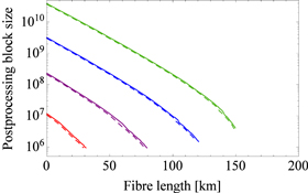
Figure 3. Postprocessing block size versus fibre length for a fixed total number of signals sent by Alice with exact intensity control, with and 12 (from left to right). The solid lines correspond to the case ξ = 0 and the dashed lines are for ξ = 0.147.


Download figure:
Standard image High-resolution image5.2. Key generation rate for the intensity-fluctuation case
In this section we evaluate the resulting secret key rate when the laser source suffers from intensity fluctuations. We study two cases: r = 0.02 and r = 0.05, where r is the deviation rate from the expected value of the intensity. The results are shown in figures 4 and 6. Here we consider that , and the term ξ takes again the values and . The security parameter is in figure 4 and in figure 6.


Figure 4. Secret key rate (per pulse) in logarithmic scale versus fibre length when the intensity fluctuation is 2%. The security parameter is and the total number of signals sent by Alice is with (from left to right). The rightmost two lines correspond to the asymptotic secret key rate with two decoy settings. The solid lines denote the case (i.e., the perfect encoding scenario) while the dashed lines show the case (which is equivalent to a phase modulation error of ). The experimental parameters are described in the main text.


Download figure:
Standard image High-resolution imageFor comparison, these two figures also show the asymptotic secret key rate when Alice and Bob use two decoy settings. In this asymptotic case, we find that the degradation on the achievable key rate, when compared to the scenario r = 0, is only about 10 km (20 km) when r = 0.02 (r = 0.05).
In the finite-key regime, however, we obtain that the presence of intensity fluctuations seems to strongly limit the key generation rate if Alice and Bob do not know their probability distribution but only know the interval where the fluctuations lie in. For instance, when and r = 0 (see figure 2) Alice and Bob can distribute a secret key over more than 100 km. However, to achieve a similar secret key rate performance when the intensity fluctuation of the source is 2% (i.e., the parameter r = 0.02) they need to exchange about signals. The main technical reason for this behaviour seems to be the fact that Azuma's inequality [36] has a relatively slow convergence speed when compared to the Chernoff bound [34] and the Multiplicative Chernoff bound [13].


As a side remark, let us mention that when r = 0.05 and we find that the achievable secret key rate is basically zero unless we increase the security parameter from to . This is illustrated in figure 6.


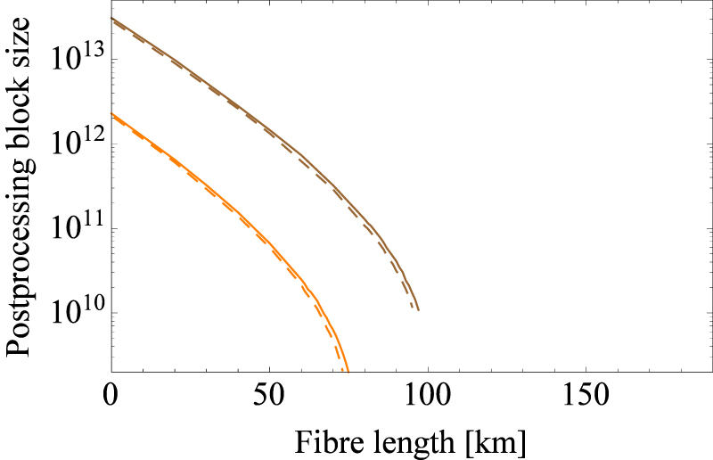
Finally, figures 5 and 7 show the postprocessing block size as a function of the distance when with for the 2% intensity fluctuation case and for the 5% intensity fluctuation case, respectively.


Figure 5. Postprocessing block size versus fibre length for a fixed total number of signals sent by Alice, with when the intensity fluctuation is 2% (from left to right). The solid lines correspond to the case ξ = 0 and the dashed lines are for ξ = 0.147.


Download figure:
Standard image High-resolution image
Figure 6. Secret key rate (per pulse) in logarithmic scale vs fibre length when the intensity fluctuation is 5%. The security parameter is and the total number of signals sent by Alice is with (from left to right). The rightmost two lines correspond to the asymptotic secret key rate with two decoy settings. The solid lines denote the case (i.e., the perfect encoding scenario) while the dashed lines show the case (which is equivalent to a phase modulation error of ). The experimental parameters are described in the main text.


Download figure:
Standard image High-resolution image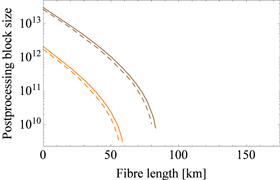
Figure 7. Postprocessing block size vs fibre length for a fixed total number of signals sent by Alice, with when the intensity fluctuation is 5% (from left to right). The solid lines correspond to the case ξ = 0 and the dashed lines are for ξ = 0.147.


Download figure:
Standard image High-resolution image6. Conclusion
In summary, we have provided explicit security bounds for the loss-tolerant QKD protocol in the finite-key regime. On the application front, our results constitute an important step towards practical QKD with imperfect light sources, in that the resulting security performance is robust against encoding inaccuracies like, for instance, optical misalignments. Furthermore, our results take into account intensity fluctuations in the light source, which is a common experimental fact. Our results highlight the importance of the stable control of the intensity modulator as well as the need for a precise estimation of its intensity, which is not often sufficiently emphasized in the experiments. On a more general outlook, it would be of great practical interest to incorporate our results into measurement-device-independent QKD (mdiQKD) [11].
Acknowledgments
We thank Lo H-K, Xu F, Kato G, Azuma K, Ikuta R, Nagamatsu Y, Takeuchi Y and Matsuki K for valuable discussions on the security analysis and parameter estimation procedure, and Yoshino K, Fujiwara M, Sasaki M, and Tomita A for fruitful discussions on practical QKD systems. AM acknowledges support from the JSPS Grant-in-Aid for Scientific Research(A) 25247068. MC thanks the Galician Regional Government (program 'Ayudas para proyectos de investigacion desarrollados por investigadores emergentes', and consolidation of Research Units: AtlantTIC), and the Spanish Government (project TEC2014-54898-R) for financial support. KT acknowledges support from the National Institute of Information and Communications Technology (NICT) of Japan (Project 'Secure Photonic Network Technology' as part of Project UQCC).
Appendix A.: Derivation of the security bound
Here we present the calculations for the security bound given by equation (2). The security analysis is based on the universal composable security framework [30].
Recall that after privacy amplification, the joint state shared by Alice, Bob and Eve is described by the following classical-quantum state

where and are the classical bit strings for the keys, associated with orthonormal states and in a Hilbert space. Here, denotes the distribution of the keys and is the quantum state of Eve's system conditioned on and . In the ideal scenario, the joint state is described by


where and is an arbitrary quantum state held by Eve. Using the security definition stated in the main text, a -secure QKD protocol satisfies


Furthermore, if the security parameter is appropriately chosen, it can be seen as the sum of errors in the correctness and secrecy, i.e., . To see this, let us introduce an intermediate state


which is just a trivial classical extension of Alice's state. Then, by using the triangle inequality property of the trace distance metric, we have

Fixing the first term on the rhs to gives


where the inequality is due to the fact that the trace distance metric is contractive under any trace-preserving operation (in our case, the partial trace operation). Similarly, by fixing the second term to we have


Therefore, fixing gives the desired decomposition.

From [32], the lower bound on the secret key length of our protocol is written as

where and are the lower bounds on the detection events of the vacuum and the single-photon emission, respectively, and is the number of rounds performing the random hashing to correct the phase error, which is equivalent to the number of bits sacrificed in the privacy amplification step of the protocol. The parameter denotes the number of bits consumed in bit error correction, and is the length of the hash that Alice sends to Bob for the error verification using the universal2 hash functions. From [7] and [33], we have that can be bounded by . Therefore, the secret key length is obtained as


where we consider η as a fixed value in this paper.
Appendix B.: Technical lemmas
In this appendix we introduce four different concentration inequalities which are used throughout this paper. First, we introduce the stochastic model that is assumed in lemmas1, 2 and 3.
Stochastic model in lemmas 1, 2 and 3. Let be a set of independent Bernoulli random variables that satisfy , and let . The expected value of X is denoted as . An observed outcome of X is represented as x.


![$\mu := E[X]={\displaystyle \sum }_{i=1}^{N}{p}_{i}$](https://content.cld.iop.org/journals/1367-2630/17/9/093011/revision1/njp518846ieqn340.gif)
Lemma 1. Chernoff bound [34].
This bound requires the knowledge of μ. It relates x with μ as

except with error probability , where the fluctuation term lies in the interval with and , where and . Here the parameter denotes the probability that . Equation (44) holds if both and are met.


![${\delta }_{{\rm{C}}}\in [-{{\rm{\Delta }}}_{{\rm{C}}},{\hat{{\rm{\Delta }}}}_{{\rm{C}}}]$](https://content.cld.iop.org/journals/1367-2630/17/9/093011/revision1/njp518846ieqn343.gif)


Lemma 2. Hoeffding bound [35].
This bound does not require the knowledge of μ. It relates μ and x as

except with error probability , where the fluctuation term lies in the interval with and , and where .


![${\delta }_{{\rm{H}}}\in [-{{\rm{\Delta }}}_{{\rm{H}}},{\hat{{\rm{\Delta }}}}_{{\rm{H}}}]$](https://content.cld.iop.org/journals/1367-2630/17/9/093011/revision1/njp518846ieqn354.gif)


Lemma 3. Multiplicative Chernoff bound [13].
This bound does not require the knowledge of μ. It combines lemmas 1 and 2 above. It uses Lemma 2 to estimate a lower bound on μ that is then basically used in combination with lemma 1. In particular, let for certain . Then, if the following two conditions are satisfied: and with , this lemma states that μ and x can be related as


except with error probability , where lies in the interval with and , and where .


![$[-{{\rm{\Delta }}}_{{\rm{M}}},{\hat{{\rm{\Delta }}}}_{{\rm{M}}}]$](https://content.cld.iop.org/journals/1367-2630/17/9/093011/revision1/njp518846ieqn365.gif)


Lemma 4. Azuma's inequality [36, 37].
Note that lemmas 1, 2 and 3 apply only to independent random variables, however, Azuma's inequality is applicable to any random variables (including dependent ones, i.e., random variables which can be correlated in any way) as long as two particular conditions (i.e., a Martingale and a Bounded difference condition (BDC), see below) are satisfied. In general, Eve's attacks can be coherent attacks, i.e., Eve can first make all the pulses sent by Alice to interact in a coherent way with an ancilla system in her hands and then measure the ancilla only after she has learned all the information distributed by Alice and Bob through the classical channel. In this general scenario, therefore, one cannot assume that each sending pulse is independent of each other. Hence, in order to analyse the security of the loss-tolerant protocol against coherent attacks in the finite-key regime, we use Azuma's inequality.
In particular, a sequence of random variables is called a Martingale if and only if for all non-negative integer l, where represents the expectation value. On the other hand, is said to fulfil the BDC if there exists such that for all non-negative integer l.

![$E[{X}^{(l+1)}| {X}^{(0)},{X}^{(1)},\ldots ,{X}^{(l)}]={X}^{(l)}$](https://content.cld.iop.org/journals/1367-2630/17/9/093011/revision1/njp518846ieqn370.gif)
![$E[\cdot ]$](https://content.cld.iop.org/journals/1367-2630/17/9/093011/revision1/njp518846ieqn371.gif)


Let us consider N trials of a random variable , where l refers to the lth trial. If is a Martingale and satisfies the BDC with then Azuma's inequality guarantees that


for any .

Let us now define the following random variable for the lth trial

where represents the actual number of events of the form observed amongst the first l trials, and is the conditional probability of having the event '1' in the uth trial conditioned on the first outcomes . In this scenario, it is straightforward to show that the random variables given by equation (48) are Martingale and satisfy the BDC with . Hence, by applying Azuma's inequality we have that


This means, in particular, that

except with error probability , where the parameter lies in the interval with and , and where .


![${\delta }_{{\rm{A}}}\in [-{{\rm{\Delta }}}_{{\rm{A}}},{\hat{{\rm{\Delta }}}}_{{\rm{A}}}]$](https://content.cld.iop.org/journals/1367-2630/17/9/093011/revision1/njp518846ieqn387.gif)


Appendix C.: Decoy-state analysis
In this appendix we first present the detail of the decoy-state analysis for the intensity fluctuation case and then we summarize all the equations for the decoy-state analysis, including those for the exact intensity control case. More precisely, we describe the estimation procedure that we use in order to obtain a lower bound on the number of vacuum contributions , and both a lower and an upper bound on the number of single-photon contributions .


C.1. Intensity fluctuation case
Here, we generalize the decoy-state method to cover the case where the source suffers from intensity fluctuations. For this, as already mentioned previously, we shall consider that Alice and Bob only know the interval where the intensity k lies.
![$[{k}^{-},{k}^{+}]$](https://content.cld.iop.org/journals/1367-2630/17/9/093011/revision1/njp518846ieqn393.gif)
We begin by calculating the mean value . Our starting point is the random variable for the ith trial when both Alice and Bob select the Z basis. This random variable takes the value 1 if Alice chooses the intensity k and, moreover, the generated signal is detected by Bob; otherwise it is 0. The term reflects the fact that may depend on all the previous trials. With this notation, can be expressed as


where Nz is the number of events where both Alice and Bob select the Z basis. The probability denotes the conditional probability that the event * occurs in the ith trial conditioned on the results obtained in the previous trials, and the term represents the event where Alice selects the intensity k and Bob detects the generated signal given that both of them have chosen the Z basis. By using Bayes rule, we can rewrite equation (51) as


where pk is the probability that Alice chooses the intensity k; n denotes an n-photon signal; pz represents the probability of selecting the Z basis; and is the probability that the event * occurs in the ith trial. For instance, is the conditional probability that Alice emits an n-photon state in the ith trial given that she has chosen the intensity k and both Alice and Bob have selected the Z basis in the ith trial. Note that in the transformation from equation (53) to (54) we have used the property of the decoy-state method i.e., .


In so doing, we obtain that is upper bounded by


Similarly, we find that

Lower bound on the number of vacuum contributions.
To obtain this bound, we first rewrite equations (55) and (56) for the cases and , respectively. We obtain the following two inequalities


Next, we multiply equation (57) by and equation (58) by , and we add both expressions. In so doing, we find that


where the second inequality holds because .

As a result, we find that is lower bounded by


To estimate the expectation values and , we use Azuma's inequality because each trial of the random variables and may depend on the previous ones.


Lower bound on the number of single-photon contributions.
Here, we first particularize equations (55) and (56) for the cases and , respectively. We have that


Next, we add both expressions and we obtain

This last equation can be rewritten as

Next, we evaluate the third term on the rhs of equation (64). This term is lower bounded by

because when the conditions , and are satisfied we have that . If we now use equation (56) for , we have that


![${({k}_{{\rm{d}}2}^{-})}^{n}-{({k}_{{\rm{d}}1}^{+})}^{n}\geqslant [{({k}_{{\rm{d}}2}^{-})}^{2}-{({k}_{{\rm{d}}1}^{+})}^{2}]{({k}_{{\rm{s}}}^{-})}^{n-2}$](https://content.cld.iop.org/journals/1367-2630/17/9/093011/revision1/njp518846ieqn422.gif)


The rhs of equation (65) can be lower bounded using the rhs of equation (66). This is so because and therefore the term in equation (65). Hence, we have that the third term on the rhs of equation (64) is lower bounded by

![$[{({k}_{{\rm{d}}2}^{-})}^{2}-{({k}_{{\rm{d}}1}^{+})}^{2}]/{({k}_{{\rm{s}}}^{-})}^{2}\lt 0$](https://content.cld.iop.org/journals/1367-2630/17/9/093011/revision1/njp518846ieqn425.gif)

That is, if we now combine equations (64) and (67) we find that

which directly gives us a lower bound on ,


Here, the lower bound on and the upper bound on and are estimated using Azuma's inequality. Upper bound on the number of single-photon contributions.


By adding equations (57) and (58), we have that

where the second inequality holds because . This means, in particular, that is upper bounded by


where the upper bound on and the lower bound on are estimated using Azuma's inequality.


C.2. Summary of the decoy-state analysis
Here, we summarize all the equations needed in the decoy-state method, including those for the exact intensity control case.
Lower bound on the number of vacuum contributions.
Let denote a lower bound on the number of events where Alice generates a vacuum state using the signal intensity and the basis setting to encode a bit value , and Bob observes the bit value when he measures the received signal using the basis .


where the parameters and are defined in a similar way like equations (9) and (10) for the exact intensity control case and like equations (20) and (21) for the intensity-fluctuation case, respectively. The probability is a lower bound on which denotes the probability that Alice selects the signal intensity setting and sends a vacuum state.


Lower bound on the number of single-photon contributions.
Let denote a lower bound on the number of events where Alice prepares a single-photon state using the signal intensity and the basis setting to encode a bit value , and Bob observes the bit value when he measures the received signal using the basis .


where the probability is a lower bound on which denotes the probability that Alice selects the signal intensity setting and sends a single-photon state.


Upper bound on the number of single-photon contributions.
Let denote an upper bound on the number of events where Alice prepares a single-photon state using the signal intensity and the basis setting to encode a bit value , and Bob observes the bit value when he measures the received signal using the basis .


where the probability is an upper bound on .


Appendix D.: Phase error rate estimation
In this appendix we explain how to derive equation (36). That is, we obtain an upper bound on the number of phase errors associated to the single-photon pulses emitted by Alice when she selects the signal intensity setting, both Alice and Bob use the Z basis, and Bob obtains a successful detection event (i.e., ). As we are interested in the phase error rate defined in the single-photon emission events and all the statistics associated with the single-photons can be estimated using the decoy state method, in the virtual protocol we only consider the cases where Alice emits single photons.

To begin with, we first review briefly the main idea that we use to derive the phase error rate; it is based on the results introduced in [21], which follow the security analysis presented by Koashi in [26] based on a complementarity argument. This method [21] requires to estimate the transmission rates (i.e., detection probabilities) that Bob would obtain if he would measure some virtual states (see equation (78) below) in a complementary basis to the key generation basis. Importantly, it turns out that these transmission rates can be written as a liner combination of the transmission rates of the actual states sent by Alice (i.e., and ). To obtain these last transmission rates, we use the detection events that correspond to basis mismatch events (i.e., the detection events where Alice and Bob's basis choices are different). From these results, we can then calculate the exact value of the transmission rates associated to the virtual states (and, therefore, the phase error rate).


Based on this idea, we expand the security analysis introduced in [21] to accommodate the finite-key size effect in the following. For this, in the security proof we consider a virtual protocol that based on the complementarity argument [26] is equivalent to the actual protocol. In the virtual scheme, Alice prepares an ancilla qubit which is entangled with the pulse that she sends to Bob. Importantly, from Eve's viewpoint both protocols are completely indistinguishable because they emit the same quantum states and announce the same classical information.
In addition, as already mentioned in the main text, here we will consider the filtered states and only for convenience, as they allow us to simplify the mathematical derivation of the transmission rates associated to the virtual states. Note that due to the action of the filter operation we can concentrate only on those states that lie in the X–Z plane rather than in the whole Bloch sphere. Most importantly, we have that the relation derived for the filtered states holds as well for the actual states because all the states, which have the same component, have the same probability of passing the filter. Indeed, one could obtain exactly the same mathematical expression for the main result of this section (see equation (103) below) without considering a filter operation, but the analysis is more cumbersome.


Let us start our analysis by introducing the following joint states, which we shall denote as . They are a purification of the signals with (see equation (32)),


where the index represents the ancilla system and the index B is the system that Alice sends to Bob. In addition, we define the state:


where the ancilla system stores the bit information. The aim of the virtual protocol is to quantify how accurately Bob can estimate Alice's measurement outcome if she would measure system in the complementarity basis (i.e., if she would use the POVM , where ). This way one can characterize the information that Eve could have obtained about the raw key [26]. Note that equation (76) can be rewritten as


where the normalized virtual states , with , are defined as


Let us now introduce some additional notation before we describe in detail the different steps of the virtual protocol. In particular, the states prepared by Alice in the virtual protocol are given by

where the shield system sh belongs to Alice's laboratory, the states have the form


and the probabilities P(c) are given by

Also, we define Bob's POVM for the Z and the X basis measurement as and , respectively. Here, the operator corresponds to the inconclusive outcome in the basis. Importantly, in the security analysis we assume that this operator is the same for both bases, i.e., . Note that this assumption is met in all those actual experiments where the detection probability for any state is independent of Bob's basis choice, and this allows us to conceptually delay Bob's measurement basis choice until he is certain to obtain a conclusive result. That is, we can consider that Bob first conducts a filter operation with Kraus operators followed by the Z or X basis measurement, which we redefine as and , respectively.


Next we present the steps of the virtual protocol in detail.
| Virtual protocol |
| Alice repeats the first step n1 times, where n1 is the number of single-photon emissions generated by Alice in the actual protocol within the set . |
| (1) Preparation |
| Alice prepares the state given by equation (79). Afterwards, she sends Bob system B over a quantum channel and delays her measurement on system sh until step 3. |
| (2) Filter operation |
| Bob performs on system B the filter operation D and, if this operation succeeds, he stores this system in a quantum memory. We will denote the set of successful filter results as . |
| (3) Collective measurement |
| Alice and Bob perform on the states in the set a collective measurement characterized by the POVM elements (see equation (84)) on the states in the set . |
| (4) Classical communication |
| Alice announces the basis choice over an authenticated public channel when the result of her measurement in step 3 is . Then, Bob announces the basis choice, also over an authenticated public channel, when the measurement outcome in step 3 is to ensure that the classical information declared in both the actual and the virtual protocols coincide (see the main text below for further details). In addition, Bob declares the value of . |
| (5) Estimation of the number of phase errors |
| Alice and Bob calculate an upper bound on the number of phase errors. This upper bound is given by |
|
where denotes the number of outcomes associated to the operator trials, and is an upper bound on . |


The size of the set (see step 2 of the virtual protocol) is upper bounded by


where the parameter is defined in appendix C. Also, the POVM elements of Alice and Bob's collective measurement are given by


These POVM elements satisfy .

It is easy to demonstrate that from Eve's viewpoint the virtual protocol described above is completely equivalent to the actual protocol. Indeed, the quantum states that Alice sends to Bob are exactly the same in both protocols. Also, both schemes declare precisely the same classical information. To see this last point, let us further clarify the fourth step of the virtual protocol. In particular, note that when the state that Alice sends to Bob in the virtual protocol is and Bob uses the basis. However, in this case, Alice and Bob announce the basis. In so doing, the actual and virtual protocols are indistinguishable. This is so because in the actual protocol the events are used to generate a secret key, i.e., in these events both Alice and Bob select, and therefore also declare, the basis. Then, the virtual protocol has to do the same declaration, otherwise it could be distinguished from the actual protocol. That is, with our definition of the virtual protocol we guarantee that it produces precisely the same classical information as the actual protocol.

![${\mathrm{Tr}}_{{{\rm{A}}}_{1}}P[{| {\tilde{\psi }}_{0(1)x}\rangle }_{{{\rm{A}}}_{1}{\rm{B}}}]$](https://content.cld.iop.org/journals/1367-2630/17/9/093011/revision1/njp518846ieqn502.gif)


Next, we present the estimation method that we use in order to upper bound the quantities using experimentally observed values. For this, we consider the sequence of random variables , with , given by


where is the conditional probability of obtaining the values in the collective measurement performed in the th trial of the third step of the virtual protocol, conditioned on the first measurement outcomes from the collective measurements . To obtain this conditional probability we use the following joint state in trials


where , and represent, respectively, Alice's prepared states in the first trials, in the th trial, and in the rest of trials.


Let denote Eve's unitary transformation on Bob's system B and on her system E. We have that


where denotes the Kraus operator which acts on system B depending on Eve's measurement outcome of her ancilla. Now we consider Alice and Bob's collective measurement. In particular, let represent the Kraus operator associated with the measurement outcome of Alice's system sh and Bob's system. Also, let denote Alice and Bob's joint measurement operator up to trials. It can be written as


We shall denote the measurement outcomes of the first trials as . Then, after Eve's intervention and conditioned on the fact of obtaining the measurement results , we have that the normalized th state of Alice's system sh and Bob's system B, which we shall represent as , is given by


where the state has the form


Here, is the trace over all systems except for the th systems sh and B. Equation (90) can be rewritten as follows:


where represents the trace over the system, the states denote an orthogonal basis for the first systems and the last systems, respectively, and


is the Kraus operator acting on the th system conditioned on the measurement outcomes .


Therefore, we obtain that the conditional probability defined in equation (85) for is given by


where , the probability , the operator , the states are defined in equation (80), and is the th conditional probability that Bob's measurement outcome in the basis is given that Alice sends him the state and the filter operation succeeds conditioned on the first measurement results. For convenience, we shall refer to as the transmission rate of .


![${T}_{{M}_{{Xs}}}^{(u| \overrightarrow{u-1})}\left[{\mathrm{Tr}}_{{A}_{1}}P[{| {\phi }^{({\rm{\Omega }})}\rangle }_{{{\rm{A}}}_{1},{\rm{B}}}]\right]$](https://content.cld.iop.org/journals/1367-2630/17/9/093011/revision1/njp518846ieqn549.gif)


![${\mathrm{Tr}}_{{A}_{1}}P[{| {\phi }^{({\rm{\Omega }})}\rangle }_{{{\rm{A}}}_{1},{\rm{B}}}]$](https://content.cld.iop.org/journals/1367-2630/17/9/093011/revision1/njp518846ieqn553.gif)

![${T}_{{M}_{{Xs}}}^{(u| \overrightarrow{u-1})}[A]$](https://content.cld.iop.org/journals/1367-2630/17/9/093011/revision1/njp518846ieqn555.gif)

If we apply Azuma's inequality (see lemma 4 in appendix B), we obtain

except with error probability , where .


By combining this result with that from equation (93), we have that

Note that the parameters , with , can be upper and lower bounded using the decoy-state method. We shall denote the failure probability of this estimation as , respectively.


As a result, we obtain bounds on that maximize the number of phase errors in the single-photon emissions within the set . They are denoted as and have the form
![${\displaystyle \sum }_{u=1}^{{N}_{1}}{T}_{{M}_{{Xs}}}^{(u| \overrightarrow{u-1})}\left[{\mathrm{Tr}}_{{A}_{1}}P[{| {\phi }^{({\rm{\Omega }})}\rangle }_{{{\rm{A}}}_{1},{\rm{B}}}]\right]$](https://content.cld.iop.org/journals/1367-2630/17/9/093011/revision1/njp518846ieqn562.gif)


When , the quantity , with , represents the transmission rate of the virtual states , with given by equation (78). This quantity can be decomposed into the transmission rate of the Pauli operators . However, for later convenience, we will decompose it as a function of , together with . Here, the states are defined in equation (31). In particular, from equation (78) we find that

![${T}_{{M}_{{Xs}\oplus 1}}^{(u| \overrightarrow{u-1})}\left[{\tilde{\rho }}_{{sx}}^{\mathrm{vir}}\right]$](https://content.cld.iop.org/journals/1367-2630/17/9/093011/revision1/njp518846ieqn567.gif)

![${\tilde{\rho }}_{{sx}}^{\mathrm{vir}}={\mathrm{Tr}}_{B}(P[{| {\tilde{\psi }}_{{s}_{x}}^{\mathrm{vir}}\rangle }_{{{\rm{A}}}_{1},{\rm{B}}}])$](https://content.cld.iop.org/journals/1367-2630/17/9/093011/revision1/njp518846ieqn569.gif)


where we have used equation (75) in the second equality and see equation (35) for the definition of .

In addition, we have that the transmission rate of can be decomposed using the Pauli operators as follows


Hence, the transmission rate of the Pauli operators can be described as

where the inverse matrix is given in equation (37).

Now, if we combine equations (99), (101) and (95), we obtain that is upper bounded by


Finally, by using the results given by equations (96)–(98), we find that


except with error probability

where is the failure probability that equation (94) does not hold for . Also, are the failure probabilities of the decoy state method i.e., the failure probabilities of the estimation of , respectively.


Appendix E.: Simulation
In this appendix we present the calculations used to obtain figures 2, 4 and 6 in the main text.
In particular, we consider that Alice sends Bob pairs of coherent states of the form , and we set Alice's (Bob's) phase modulation error to (). Also, we assume a Gaussian distribution for the intensity fluctuations of the laser within an interval . That is, we consider that the probability density function of the fluctuations is given by , where is the desired value (e.g., , and ), the dispersion has the form , and the normalization factor is such that .


![$[{k}^{-},{k}^{+}]$](https://content.cld.iop.org/journals/1367-2630/17/9/093011/revision1/njp518846ieqn586.gif)
![${p}_{{\rm{G}}}(k)=A\mathrm{exp}[{-(k-\mu )}^{2}/2{\sigma }^{2}]$](https://content.cld.iop.org/journals/1367-2630/17/9/093011/revision1/njp518846ieqn587.gif)


Calculation of the parameters .

For this, we need to obtain for all . Afterwards, we simply apply the procedure described in section 4.1 (for the exact intensity control case) and in section 4.2 (for the intensity fluctuation case).


We consider that the total number of pulses sent by Alice using the intensity setting is given by , where denotes the total number of transmissions until the conditions in the Sifting step of the protocol are met. The total system loss includes the channel loss and the detection efficiency of Bob's detectors. The conditional probability that Bob obtains the bit using the basis given that Alice sends him a bit encoded with the intensity and also in the basis can be written as


The conditional probability that Bob interprets the bit value (after a random assignment of double click events to single clicks events) when he uses the basis given that Alice sends him a pulse with the intensity , prepared in the basis, and encoding the bit value is written as


To simulate the misalignment in the optical system we transform this probability as


In so doing, we obtain

The bit error rate in the basis when Alice sends Bob a pulse using the signal intensity is given by


Calculation of the parameter .

According to equation (36), we have that is upper bounded by


To obtain we first calculate the probability that Bob obtains the bit with the basis given that Alice sends him a pulse of intensity using the basis and encoding the bit value . For this, we have that


Then, by using equation (109) we find

Finally, we include the effect of the misalignment in the optical systems. That is, we transform as


The number is therefore given by


Next, we calculate . For this we need to obtain . We have that the probability that Bob obtains the bit with the basis given that Alice sends him a pulse of intensity , prepared in the basis, and encoding the bit value is given by


In this scenario the probability has the form


and therefore the quantity can be written as


Footnotes
- 6
In the asymptotic limit of an infinitely long key, the problem of intensity fluctuations in decoy-state QKD has been considered in [29].
- 7
Note that the recent work [31] shows that discrete phase randomization is sufficient for the BB84 protocol.
- 8
Note that in those scenarios where Alice knows the exact probability distribution of the fluctuations then the conventional decoy-state method can be directly applied.
- 9
Note that this random assignment is not mandatory, and Bob can always choose a particular bit value, say 0, for as this preserves the basis-independence detection efficiency condition.
- 10
Note that this filter operation is just a mathematical tool for the security analysis, and it does not need to be implemented in the actual experiments. It is mainly used to simplify the estimation of the transmission rates of some virtual states that are needed to calculate the phase error rate of the protocol (see appendix D). Such derivation could be performed as well without considering such filtered states, but the analysis is more cumbersome.
