


Abstract
A key component in calculations of exchange and correlation energies is the Coulomb operator, which requires the evaluation of two-electron integrals. For localized basis sets, these four-center integrals are most efficiently evaluated with the resolution of identity (RI) technique, which expands basis-function products in an auxiliary basis. In this work we show the practical applicability of a localized RI-variant ('RI-LVL'), which expands products of basis functions only in the subset of those auxiliary basis functions which are located at the same atoms as the basis functions. We demonstrate the accuracy of RI-LVL for Hartree–Fock calculations, for the PBE0 hybrid density functional, as well as for RPA and MP2 perturbation theory. Molecular test sets used include the S22 set of weakly interacting molecules, the G3 test set, as well as the G2–1 and BH76 test sets, and heavy elements including titanium dioxide, copper and gold clusters. Our RI-LVL implementation paves the way for linear-scaling RI-based hybrid functional calculations for large systems and for all-electron many-body perturbation theory with significantly reduced computational and memory cost.

Content from this work may be used under the terms of the Creative Commons Attribution 3.0 licence. Any further distribution of this work must maintain attribution to the author(s) and the title of the work, journal citation and DOI.
1. Introduction
With advances in high-performance computing and improved numerical algorithms, the predictive power of first-principles electronic-structure theory is increasing in terms of accuracy and tractable system size. Density-functional theory (DFT) using (semi-)local functionals has excelled because of a very favorable combination of computational efficiency and reasonable accuracy in solid-state theory and quantum chemistry. However, it is well documented that conventional DFT methods are not sufficient to properly describe certain types of binding interactions [1–6]. It is often necessary to use hybrid functionals [7, 8] or even higher-level methods like second-order Møller–Plesset perturbation theory [9] (MP2), GW methods [10, 11] or the random-phase approximation (RPA) and beyond [12–14] to accurately treat e.g. cohesive energies, van der Waals interactions or reaction-barrier heights.
For hybrid functionals and more sophisticated treatments of the electronic exchange and correlation a major computational bottleneck is the evaluation of the two-electron repulsion integrals for orbitals


The notation refers to the Coulomb interaction between the functions indexed by a and b, respectively, throughout the paper. In particular, we have and where .


Upon replacing the orbitals by their expansions in a chosen set of basis functions , equation (1) transforms into a sum over four different basis function indices. The approach for evaluating these integrals largely depends on the basis set. For Gaussian or plane wave basis sets these integrals are given analytically. For numeric atom-centered orbital [15–23] (NAO) basis sets on the other hand, these integrals with four different atomic positions , often called four-center integrals, have to be evaluated by explicit integration.


A straightforward approach for basis sets with analytical solutions is possible, but due to the integrals this leads to unfavorable execution times for large systems. For NAOs, on the other hand, no analytical solution exists. Computing these integrals on the fly becomes intractable as the system size grows. Precomputing them is also out of the question due to the memory and communication requirements for storing and reading this matrix with entries.


A widely used approach to alleviate the computational time requirements of the four-center integral evaluation is the 'resolution of identity' (RI), also known as 'density fitting' [24–30]. The central idea is to expand orbital products into an auxiliary basis :


This approach represents the four-index matrix in terms of three- and two-index ones and is therefore better suited to be precomputed and stored. The auxiliary basis functions can either be predefined or calculated at runtime. The most commonly used variant is the 'RI-V' scheme [24, 29–31], which determines the expansion coefficients by directly minimizing the errors in the four-center integrals. This scheme has the advantage that the error in the four-center integrals is quadratic in the error of the actual RI expansion [24, 25]. This approximation, together with the fact that the total energy is stationary with respect to the expansion coefficients, makes the RI-V a 'robust variational' scheme [25].

Our group has successfully applied the RI to NAOs and shown it to be a reliable and robust approach [32]. Additionally, a general procedure for the construction of the auxiliary basis was presented that is particularly accurate for on-site products of atomic orbitals, which carry the bulk of the total energy. While RI expansions for any atomic basis set are particularly efficient for small systems, the scaling behavior, both in terms of computational time and memory usage, is problematic because of the nonlocal nature of expansions based on the Coulomb metric [33]. (See equations (6) and (7) below.) In principle, this nonlocality is artificial as a local quantity like the product of two localized orbitals should not need expansion functions arbitrarily far away, and it makes the application to large or even periodic systems [34] impractical or even impossible.
There are several previous studies exploring ways to limit the number of nonvanishing expansion coefficients. For example Reine et al replaced the global Coulomb metric with a localized one [35]. Sodt et al followed a more pragmatic approach by restricting the expansion of a basis function product to the subset of those auxiliary basis functions which are centered within a sphere around one of the two basis function centers [36, 37]. Pisani et al followed a similar approach with a more general fitting domain for local MP2-calculations in periodic systems [38, 39]. Recently, Merlot et al presented a localized RI, which uses only auxiliary basis functions centered on the two centers of the expanded basis functions as a starting point [40]. To reach a reasonable accuracy, they then applied a Cholesky decomposition scheme to converge the integration accuracy by adding further auxiliary functions along the connection line between the two centers. Even more localized density fitting approaches were already known in the early days of computational quantum chemistry. Of particular interest for the present work is the limited expansion of diatomic overlap (LEDO) of Billingsley and Bloor [24, 41]. In this work, the authors expanded products of Slater type orbitals on different atoms in the on-site products of these two atomic centers.
In addition to using localized variants of the RI approach, several other techniques for the evaluation of four-center integrals have been investigated in the literature. Delley evaluated the products of molecular orbitals on an atom-centered numerical grid and used multipole techniques to solve the Poisson equation [42]. Already in the early 1980s [43], Talman showed how to use Fourier space techniques [44, 45] to spherically expand NAO products around a point between the two orbital centers, and how to efficiently calculate the Coulomb interactions between such expansions [43, 46]. Recently, a more efficient way of spherically expanding orbital products based on Legendre integration was published by the same author [47]. Foerster showed how to construct a compact auxiliary basis a posteriori from Talman's expansion [43, 46] for a given atom pair by means of a singular value decomposition [48, 49]. In contrast to our strictly atom-centered approach, this work employs bond-centered auxiliary basis sets. Another technique is the expansion of the NAOs in terms of a Gaussian function set, which is implemented in the SIESTA code [50, 51]. While this strategy has the advantage of offering an analytic solution, each NAO must be fitted by several Gaussians, which partially undoes the benefits of the compactness of NAO basis sets. Most of these studies aim at computing the four-center integrals directly, while the aim of the RI-approach is to compute a set of intermediate expansion coefficients that can be stored in memory. Some of the integration techniques developed by Talman are employed in our work as well.
In the present paper we demonstrate an approach that is similar to LEDO, but gives accurately converged total energies for NAOs, for Hartree–Fock (HF) and hybrid DFT functionals, as well as for correlation methods like MP2 and RPA. A similar atomic RI strategy has recently been implemented for Gaussian-type orbitals (GTO) by Manzer et al [52]. In contrast to our work, they only apply their new algorithm to the exchange integrals of the SCF-cycle at present.
Our method has recently been applied in a linear-scaling implementation of hybrid density functionals for periodic systems [34] and allows for simple nuclear derivatives, used, e.g., in a corresponding implementation of the stress tensor for hybrid density functionals [53].
We will introduce our method, which is implemented in the Fritz Haber Institute ab initio molecular simulations package (FHI-aims [16, 54]), as a localized modification of our global fitting approach reported in [32]. In section 2 we briefly review our RI scheme and introduce our new localized variant. Section 3 shows an extensive study on the convergence and accuracy for different methods, and in section 4 we compare the computational scaling with our RI-V implementation. Finally, we summarize our results and draw conclusions in section 5.
2. Theory
The basic RI implementation in FHI-aims is described extensively in [32]. We here briefly recapitulate the key equations before proceeding to the localized expansion. Finally, we explain how the localized variant can be adapted in a controlled way to further increase the accuracy which is required to minimize the linear error terms arising in our localized approach (see below).
2.1. Global expansion
The nonlocal exchange operator as part of the generalized Kohn–Sham or Fock matrix is defined by

where Djk is the one-particle density matrix and are four-center integrals of basis functions , analogous to the four-center integrals defined in equation (1) for the orbitals .


In the RI, orbital products are expanded in a set of auxiliary basis functions :


to give the approximated product . The two-electron integrals (equation (1)) are then reduced to:


Several strategies have been proposed to determine the expansion coefficients . The most common variant is known as 'RI-V'. This approach directly minimizes the error of the four-center integrals. Whitten has shown [24] that this can be achieved by minimizing the Coulomb integral of the fitting error :


The minimization problem then leads to a system of linear equations:

yielding the expansion coefficients and the approximated four-center integrals:


The four-index matrix we started with is now represented by only two- and three-index objects, implying a significant advantage in terms of memory requirements and computational time. Furthermore, the error of the approximated four-center integrals is quadratic in the residual of the fitted orbital product [25].

Unfortunately, the Coulomb kernel is long-ranged, so that and are neither sparse nor short-ranged except when the overlap between and vanishes. The consequence is a canonical computational and memory scaling with system size for the precomputed expansion coefficients . It can be reduced to memory scaling by taking the vanishing overlaps into account, but in both cases there is a large prefactor in actual computations. The formal scaling for the exchange matrix construction is not reduced by the RI approach, unless density matrix screening techniques [55] are used when the exchange matrix is computed. Since the Coulomb metric distributes the expansion coefficients for any given (localized) density over all auxiliary basis functions in the system, O(N) scaling can no longer be achieved for the exchange operator.


2.2. Construction of the standard auxiliary basis
In our implementation [16, 32], all atom-centered basis functions are defined as:


where uskl(r) is a radial function with index k and angular momentum l for species s and denotes a spherical harmonic. Both the radial part and the spherical harmonics are real-valued functions. The basis functions are constructed numerically and are subject to a cut-off potential Vcut(r), which enforces a smooth decay to zero of the basis functions outside the relevant range [16]. The construction of the confined basis functions is described in detail in equations (8) and (9) of [16]. In short, all radial functions in FHI-aims are solutions to:


Our auxiliary basis functions are not predefined, but rather derived from the basis set used to expand the orbitals . Our construction scheme for the ensures an exact reproduction of those integrals with basis functions centered at the same atom, which account for the major part of the total energy. We therefore construct our auxiliary basis set such that it contains all on-site products of basis functions explicitly. Specifically, the auxiliary basis set can be derived from two different underlying basis sets:


- OBS: the standard orbital basis set used to expand the Kohn–Sham orbitals of the DFT calculation
- OBS+: an enhanced OBS with additional functions, which are used only for the construction of the functions

In figure 1 the auxiliary basis construction is illustrated as a flowchart. For each atom species s in the system we compute all on-site products of the radial basis functions uskl(r). These products are then orthogonalized with a Gram–Schmidt scheme. A radial product is accepted as a new radial auxiliary basis function in a given angular momentum channel if the norm of its projection orthogonal to the already accepted functions is larger than a small value (for RI-V: 10−2 for atoms with , 10−3 for atoms with and 10−4 for all other elements).


Figure 1. The construction of the auxiliary basis in FHI-aims: starting from the orbital basis set, the on-site products of two radial functions (with subscripts for species, index and angular momentum) are orthonormalized. The product of the resulting function with spherical harmonics represents the auxiliary basis functions. One important feature of this approach is that we can add further radial functions (gray box) to the orbital basis set, which are only used during this procedure and do not influence the performance of the orbital basis in any way.

Download figure:
Standard image High-resolution imageThe choice of this parameter controls the size of the auxiliary basis and thus the expansion accuracy [32]. The accepted products are then multiplied with each spherical harmonic which satisfies the Clebsch–Gordon condition to obtain the . The maximum angular momentum of any basis function in the OBS or OBS+ of a given species, lsmax, thus also controls the maximum angular momentum of any basis function in the auxiliary basis set, . For each species s the maximal angular momentum of the product functions can be capped to reduce the size of the auxiliary basis, but this comes at the price of a reduced accuracy. In this work, we do not restrict lscap in any way for either RI-V or for our new localized RI. For production calculations beyond this work, we find that lscap should never be reduced for the localized RI. For RI-V, we find that lscap = 5 for elements below Xe (Z = 54) and lscap = 6 for heavier elements are sufficient for well-converged results.


2.3. Construction of the enhanced auxiliary basis
Our standard procedure for the construction of the has the advantage of producing an atom-centered auxiliary basis that automatically adapts itself to the orbital basis set and that yields a particular high accuracy for on-site products. The off-site products on the other hand are not included in the auxiliary basis set and therefore will not be expanded exactly. To obtain accurate results for these integrals too, we must use a sufficiently large auxiliary basis set. This can be readily achieved with our construction scheme by enhancing the OBS with additional functions, which are used only for the construction of the auxiliary basis set, as shown by the gray box in figure 1. This enhanced OBS is labeled OBS+ and yields a larger set of functions. Since the auxiliary basis is constructed at the species level, this approach will add the additional auxiliary basis functions to each atom of the affected species. The choice of additional basis functions will be discussed in detail in section 3.1.


2.4. Localized expansion
As our aim in this work is to reduce the number of expansion coefficients substantially, we restrict the expansion coefficients to be non-zero only if the auxiliary function μ is centered at one of the two atoms at which the basis functions i and j are centered. This restricted expansion of the product (centered on atoms I and J) can be written as


where denotes the set of all auxiliary functions centered at atom I or atom J, as depicted in figure 2.


Figure 2. The localized version of the RI approach: the function product is to be expanded in terms of the auxiliary basis set centered at atom I or J. Auxiliary basis functions centered on other atoms, like on atom K, are not used.


Download figure:
Standard image High-resolution imageSince the RI-V prescription has proven to be a robust scheme, we use the same minimization target for our localized variant. In practice, this means that we minimize the Coulomb self-repulsion of the residual from the restricted expansion:


with respect to variations in . The minimization condition then leads to a set of linear equations similar to the one for RI-V (equation (5)):


for the coefficients . Both indices μ and ν are restricted to the subset . As a consequence, the system of linear equations can be decomposed into a set of subproblems, one for each atom pair. Finally, the expansion coefficients and four-center integrals can be written as


with where is a square matrix with the entries for . The dimension of is therefore with NauxIJ being the number of centered on atoms I and J, which is only a small fraction of the total number of auxiliary basis functions Naux. If we now insert equation (12) into equation (4), we obtain


where the sums are restricted to the subset because of equation (12). We name this expansion 'RI-LVL' after the matrices occurring in equation (13).

One advantage of this scheme lies in the fact that the size of the local Coulomb matrices required for each atom pair is independent of the system size. Their number initially increases quadratically, but with increasing system size the number of relevant pairs scales linearly. Due to the cubic scaling of matrix inversions, the inversion of several local Coulomb matrices becomes favorable for large systems compared to the single inversion of a global Coulomb matrix.

Furthermore, we no longer need the full three index object , but only the parts relevant for equation (12). Additionally, the calculation of the remaining three-index integrals is simplified within RI-LVL because the center of μ is either I or J. The product of the Coulomb potential of with, say, is a simple superposition of atom-centered functions, whose overlap with can be calculated in Fourier space using the methods suggested by Talman [43, 46] as described in [32]. Together with the strong reduction in the number of these integrals the computational time can be reduced to an extent where it is small compared to the other parts of the calculation.


2.5. Error analysis
The following exact relation of four-center integrals and their RI approximations

is important for assessing the accuracy of RI schemes. Here, are the exact products, their RI approximations and are the residuals. The first term is the straightforward RI expansion used so far. The next two terms are linear in the residual, whereas the last is quadratic in the residual.


In RI-V, the minimization criterion for the residual equation (5) can be rewritten as . Since all approximated products are expanded in the , the linear terms must vanish in RI-V.


The localized version, on the other hand, only enforces this condition for those which are centered on the same atoms as the basis function composing the product. Therefore, the linear terms will only vanish for those integrals for which , where the capital letters denote the atom index of the corresponding orbital basis function. For all other integrals, the error is linear in the residuals.


Some localized RI-schemes alleviate this error by using the robust Dunlap correction[25]. Localized schemes can be extended to yield quadratic errors in the residual by including the linear error terms from equation (14) in (13):

In RI-V, all of these three terms are identical and therefore reduce to the previously used formula (equation (7)) for the four-center integral. This expression has a few drawbacks: to calculate the correction terms, all of the three-index Coulomb integrals are required. (This also includes those for which is not centered on the same atom as or .) Since the sparsity in the three-index Coulomb integrals is the key to our memory and computational time savings, this correction would undo most of our achievements. Furthermore, it also has been recently demonstrated [40] that this expression can lead to serious convergence problems in rare cases, because the matrix for the approximated four-center integrals is not necessarily positive semi-definite. Since negative eigenvalues correspond to attractive electron–electron interactions, the usual safeguards to ensure SCF convergence will lead to a high ratio of rejected steps, slowing SCF convergence down or preventing convergence at all.


Due to these drawbacks, we do not employ the Dunlap correction for our localized scheme. As we will show in section 3, the combination of a localized RI from equation (13) with localized NAOs nevertheless reproduces the results obtained from RI-V with essentially exact accuracy while significantly decreasing the computational requirements. The key step is an appropriate enhancement of the auxiliary basis itself.
3. Results
In this section we demonstrate that our RI-V implementation is a reliable benchmark for RI-LVL by comparing it to the GTO based NWChem [56] code that does not employ the RI approximation. In this step, we use Gaussian-type functions in FHI-aims so that we can perform the comparison for exactly the same basis functions. We then evaluate the accuracy for RI-LVL for HF [57] and second-order Møller–Plesset perturbation theory [9] (MP2), as well as for the PBE0 [8] hybrid functional and the RPA [12–14].
As explained in the previous section, we enhance the normal OBS with additional functions to improve the accuracy of the resulting . Throughout this article we only add hydrogen-like functions with the minimal principal quantum number for the given angular momentum, i.e. nodeless radial functions. For these functions, we have in equation (9). In the following, spd(z = x) will denote the enhancement of the OBS, i.e. which additional functions OBS+ contains, as described in section 2.2. spd indicates the added angular momentum channels (s, p, d, f etc) and z = x denotes the effective charge parameter of the added hydrogenic basis functions. Neither for RI-V nor RI-LVL we did impose any constraints on the maximal angular momentum () of the .


Individual total energy values for all structures in all benchmark sets used for each method can be found in the supporting information (SI).
3.1. HF and MP2 calculations
To demonstrate the general applicability of our approach, we first discuss HF and MP2 total energies for RI-V and RI-LVL in FHI-aims using Gaussian basis sets and compare them to the results obtained with NWChem. We then show that the same degree of accuracy can be obtained using the NAO basis functions of FHI-aims.
3.1.1. Gaussian type orbitals
To establish a valid reference for our comparison between RI-V and RI-LVL, we first calculate total energies for the molecular geometries compiled in the S22 test set of Jurečka and coworkers [58] with the Gaussian basis set cc-pVTZ [59]. This test set contains 22 weakly bonded dimers with 6–30 atoms per dimer, ranging from the water dimer to adenine–thymine complexes. This test set allows us to test total energies of molecular systems as well as weak binding energies, which usually require RPA or MP2 for an accurate description. Figure 3 shows the total energy errors for all molecular dimers and table 1 shows the root mean square deviation (RMSD) and maximum absolute value (MAX) for the error per atom (not counting hydrogens) and the systemwide error. The results show that the RI-V implementation in FHI-aims is reliable and accurate [32], yielding deviations in total energy of less than 1 meV per system for HF calculations. Also the MP2 corrections, which are more sensitive to the accuracy of the four-center integrals, are of similar quality, with a RMSD below 0.2 meV. Our RI-V implementation is therefore a suitable reference choice to benchmark RI-LVL and will be employed as such throughout the rest of this work.

Figure 3. Total errors in the total energy computed with FHI-aims using RI-V and RI-LVL, compared to NWChem. The upper panel shows the errors of Hartree–Fock calculations and the lower panel shows the errors of the MP2 correction in the S22 test set using the cc-pVTZ Gaussian basis set. 'RI-LVL+aux' uses an additional g-function for constructing the auxiliary basis. The area highlighted with the light green background is plotted using a linear y axis, the non-coloured area corresponds to a logarithmic y axis where only the 2nd and 5th intermediate grid lines are plotted. See SI for details.
Download figure:
Standard image High-resolution imageTable 1. Root mean square deviation and maximum (absolute) value of the total energy error (total and per atom, not counting hydrogens) of RI-V in the S22 test set compared to NWChem using the cc-pVTZ basis set. (See also figure 3.)
| HF | MP2 | ||||
|---|---|---|---|---|---|
| (meV) | RMSD | MAX | RMSD | MAX | |
| RI-V | Total | 0.383 | 0.716 | 0.182 | 0.445 |
| per atom | 0.038 | 0.082 | 0.028 | 0.085 | |
| RI-LVL | Total | 9.129 | 18.423 | 168.995 | 440.565 |
| per atom | 0.743 | 1.062 | 11.432 | 29.371 | |
| RI-LVL +aux | Total | 0.527 | 0.936 | 0.581 | 1.144 |
| per atom | 0.051 | 0.087 | 0.055 | 0.111 | |

Table 2. RMSD and maximum absolute errors for Hartree–Fock calculations in the S22 test set using the RI-V method with tier 2 basis sets. The functions listed under 'aux basis additions' are added to those from the bare basis set when the product basis is constructed.
| (meV) | ||||
|---|---|---|---|---|
| Aux basis | Per atom | Systemwide | ||
| additions | RMSD | MAX | RMSD | MAX |
| s(z = 1) | 0.005 | 0.016 | 0.040 | 0.124 |
| sp(z = 1) | 0.009 | 0.024 | 0.090 | 0.201 |
| spd(z = 1) | 0.011 | 0.020 | 0.119 | 0.318 |
| spdf(z = 1) | 0.023 | 0.064 | 0.341 | 1.219 |
| spdfg(z = 1) | 0.154 | 0.367 | 2.320 | 6.976 |


The straightforward localized RI on the other hands yields significantly higher errors of up to 29.5 meV/atom (up to 440 meV total error) for MP2 calculations and also gives less accurate results for HF, although the discrepancies there are less dramatic. However, the plot also shows an additional set of curves, labeled 'RI-LVL+aux', which corresponds to RI-LVL with an enhanced auxiliary basis (using a single hydrogenic g function with z = 6). This data set shows that RI-LVL yields an accuracy similar to RI-V provided a suitable chosen OBS+ and thus auxiliary basis set is chosen. We will discuss the choice of OBS+ in detail below. (The interested reader is referred to appendix

In addition to the S22 test set we also investigated the performance of our new method in the larger G3 test set [60]. This test set contains 223 molecules composed of first and second row elements. As in the S22 case we used NWChem as a reference for our RI implementations. The results for HF and MP2 total energies are shown in figure 4. We have not included the 28 dimer systems in the statistical analysis, because RI-V and RI-LVL are the same procedures for dimer systems.

Figure 4. RMSD and MAX errors in the total energy computed with FHI-aims using RI-V and RI-LVL, compared to NWChem. The left side shows the errors of Hartree–Fock calculations and the right side shows the errors of the MP2 correction in the G3 test set using the cc-pVTZ Gaussian basis set. 'RI-LVL+aux' uses an additional g-function for constructing the auxiliary basis. The dimer-systems from the test set were excluded because they are of little interest for the accuracy analysis of the RI-LVL. See SI for details.
Download figure:
Standard image High-resolution imageOverall, RI-V achieves a very good accuracy with an RMSD of the total energy of about 1 meV. As was already the case in the S22 test set, RI-LVL itself performs worse and yields errors with tens or even hundreds of meV magnitude. However, enhancing the auxiliary basis with the same functions we used in the S22 test set, we can again recover the same accuracy as RI-V. A few test cases still exhibit total energy errors up to 5.5 meV. For all these cases the RI-LVL results lie exactly on top of the RI-V results, which is a strong indication that these errors are not specific to RI-LVL. It should also be noted that almost all the outliers contain chlorine atoms.
3.1.2. Numeric atom-centered orbitals
For the remainder of the article, we will return to the NAO basis sets and focus on improving the accuracy of RI-LVL. For HF calculations we use the standard tier 2 basis sets [16] with tight settings. For MP2 calculations, on the other hand, we use the recently developed valence correlation consistent NAO basis sets [61].
As seen in figure 3, our standard procedure to construct the yields sufficiently accurate total energies at the HF level. However, it does not suffice to converge MP2 total energies with our localized RI. A straightforward way to deal with this error is to increase the size of the auxiliary basis. This is achieved by using OBS+ instead of OBS for the construction of the auxiliary basis set, as discussed in section 2.3.

We first show that our reference is well converged with respect to the auxiliary basis by enhancing the original OBS with functions of increasing angular momentum (see upper panel in figure 5). Then we apply the same systematic approach to RI-LVL and finally we demonstrate that an OBS+ with only a single extra g function (see lower panel in figure 5) is sufficient.

Figure 5. Radial shape of the employed basis functions. The upper panel shows basis functions with different angular momentum and constant effective charge z = 1. The lower panel shows 5g radial functions with different effective charges z. The dashed line in both panels shows the onset of the basis confining potential.
Download figure:
Standard image High-resolution imageTable 2 njp518333t1 shows the impact of this enhanced on the HF total energies calculated with RI-V. Even if the auxiliary basis set is significantly enlarged with extended functions having high angular momenta, the change in total energy is below 0.16 meV per atom (max 0.37 meV).

Figure 6 shows that the error of RI-LVL systematically converges with increasing auxiliary basis set size. By including additional radial functions with angular momentum s, p, d, f and g in the auxiliary basis construction the RMSD of the total energy per atom can be reduced from 1.9 to 0.13 meV. Therefore, the error introduced in a HF calculation by using the local RI approximation can be controlled systematically by adding higher angular momenta to the and decreases to a negligible value.

In figure 6 it can be seen that the addition of f and g functions has the largest impact. It turns out that a single g function is already sufficient. As shown in table 3, the accuracy of the hierarchical approach can even be surpassed if we alter the effective charge that defines the added g function, but the general quality of the result is unaffected by the choice of the effective charge. The reason why the results do not depend strongly on the shape (see lower panel of figure 5) of the added function is the basis-confining potential (see equation (9)). As can be seen in figure 5, the onset and peak position of the radial function depends on the effective charge, but their behavior in the outer regions is similar. Without the confinement potential, the radial functions would extend further and the results would probably show a significant dependence on the effective charge.

Figure 6. Convergence of the HF total energy error of the RI-LVL approximation with increasing auxiliary basis set size. The difference between the RI-LVL calculations and the RI-V reference using the pure tight (tier 2) basis set is shown. The black line shows the performance of the OBS+ with a single g-function(z = 1), which we consider sufficient for production calculations (see also table 3).
Download figure:
Standard image High-resolution imageTable 3. RMSD and maximum absolute errors for Hartree–Fock calculations in the S22 test set using the RI-LVL method with tier 2 basis sets. The functions listed under 'aux basis additions' are added to those from the bare basis set when the product basis is constructed.
| HF RI–LVL | (meV) | |||
|---|---|---|---|---|
| Aux basis | Per atom | Systemwide | ||
| additions | RMSD | MAX | RMSD | MAX |
| None | 0.594 | 1.891 | 3.959 | 6.432 |
| spdfg(z = 1) | 0.052 | 0.124 | 0.493 | 1.466 |
| g(z = 1) | 0.066 | 0.153 | 0.633 | 1.799 |
| g(z = 2) | 0.059 | 0.137 | 0.567 | 1.663 |
| g(z = 3) | 0.054 | 0.127 | 0.533 | 1.590 |
| g(z = 4) | 0.053 | 0.125 | 0.514 | 1.544 |
| g(z = 5) | 0.053 | 0.123 | 0.491 | 1.454 |
| g(z = 6) | 0.047 | 0.107 | 0.465 | 1.305 |
| g(z = 7) | 0.046 | 0.098 | 0.462 | 1.226 |

We also investigated the use of RI-LVL in MP2 calculations. For these calculations we use the recently developed compact NAO based valence correlation consistent basis sets [61] that facilitate an extrapolation to the complete basis set limit.
As can be seen from table 4, RI-V with the 3Z-version of these basis sets is essentially insensitive to an enlarged auxiliary basis set, yielding at most a change of 0.1 meV per atom compared to the pure basis set. In the following analysis, RI-V with the NAO-VCC-3Z basis set with the standard auxiliary basis set will therefore be used as the reference to benchmark the MP2 results.
Table 4. RMSD and maximum absolute errors for MP2@HF in the S22 test set using the RI-V method with the NAO-VCC-3Z basis set. The functions listed under 'aux basis additions' are added to those of the bare basis set when the product basis is constructed.
| MP2@HF RI–V | (meV) | |||
|---|---|---|---|---|
| Aux basis | Per atom | Systemwide | ||
| additions | RMSD | MAX | RMSD | MAX |
| s(z = 1) | 0.003 | 0.008 | 0.031 | 0.076 |
| sp(z = 1) | 0.013 | 0.045 | 0.050 | 0.123 |
| spd(z = 1) | 0.012 | 0.036 | 0.066 | 0.126 |
| spdf(z = 1) | 0.011 | 0.027 | 0.076 | 0.144 |
| spdfg(z = 1) | 0.031 | 0.098 | 0.494 | 1.856 |

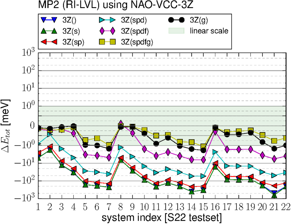
Figure 7 shows the accuracy for MP2 using the same representation as figure 6 did for HF. In essence, we find the same results as for HF: if functions up to angular momentum channel f are included in OBS+, the error can be reduced to 0.43 meV per atom (6.52 meV for the system) at most, while an additional g function reduces the error even further to at most 0.11 meV per atom (1.15 meV for the system). As for HF and the tier basis, the accuracy of the hierarchical approach can also be achieved with fewer auxiliary basis functions. Table 5 shows that a single g-function reduces the total energy error to the same order of magnitude as the addition of s, p, d, f and g functions. As for HF we find that the general quality of the results is insensitive to the variation of the effective charge, but can be fine-tuned to yield errors slightly below those of the systematic approach.

Figure 7. MP2 total energy errors of the RI-LVL calculations using the NAO-VCC-3Z basis set with additional auxiliary basis functions, compared to the RI-V calculation with the pure basis set. The black line shows the performance of the OBS+ with a single g-function (z = 1), which we recommend for production calculations.
Download figure:
Standard image High-resolution imageTable 5. RMSD and maximum absolute errors for MP2@HF in the S22 test set using the RI-LVL method with the NAO-VCC-3Z basis set. The functions listed under 'aux basis additions' are added to those of the bare basis set when the product basis is constructed.
| MP2@HF RI–LVL | (meV) | |||
|---|---|---|---|---|
| Aux basis | Per atom | Systemwide | ||
| additions | RMSD | MAX | RMSD | MAX |
| None | 13.919 | 32.970 | 195.751 | 494.545 |
| spdfg(z = 1) | 0.047 | 0.104 | 0.548 | 1.141 |
| g(z = 1) | 0.063 | 0.111 | 0.859 | 2.006 |
| g(z = 2) | 0.064 | 0.114 | 0.881 | 2.003 |
| g(z = 3) | 0.059 | 0.104 | 0.814 | 1.879 |
| g(z = 4) | 0.054 | 0.097 | 0.737 | 1.780 |
| g(z = 5) | 0.036 | 0.070 | 0.483 | 1.324 |
| g(z = 6) | 0.028 | 0.074 | 0.364 | 1.035 |
| g(z = 7) | 0.046 | 0.082 | 0.610 | 1.384 |

3.2. PBE0 and RPA
To demonstrate RI-LVL's broad range of applicability, we also performed calculations with the PBE0 exchange-correlation functional [8] and the RPA [12–14].
For PBE0 we use tier 2 basis sets, as we did for HF. For converged RPA total energies, larger NAO basis sets are required [62] and we thus use the NAO-VCC-3Z basis set again. As in the cases of HF or MP2, for PBE0 the RI-V shows no significant dependence on the added auxiliary basis functions (data not shown). When the product basis is enhanced with additional auxiliary functions, the RI-LVL results can be controlled and converged in a systematic way. In contrast to the previous HF calculations (see figures 3 and 6), we find that no OBS+ is needed to obtain accurate results with PBE0. This has two reasons: first, compared to the cc-pVTZ basis set used in figure 3 the tier 2 basis already contains a g-function in the orbital basis set. (See table 10 for more details on the tier basis sets and table 12 for an example of how the auxiliary basis set is enhanced by the additional g function.) The second reason is that PBE0 only contains 25% exact exchange, which reduces the total energy error accordingly, when compared to the tier 2 HF calculations.
Table 6 shows the relevant errors for the hierarchical enhancement of the auxiliary basis. As for HF, we can significantly reduce the RMSD and maximal value of the total energy error per atom, in this case by more than one order of magnitude from 0.19 to 0.02 meV. If the auxiliary basis is only enhanced by a single g-function, we find results similar to those from the HF analysis: the effective charge of extra function in the OBS+ has no significant impact on the achieved accuracy.
Table 6. RMSD and maximum absolute errors for PBE0 in the S22 test set using the RI-LVL method with the tier 2 basis set. The functions listed under 'aux basis additions' are added to those of the bare basis set when the product basis is constructed.
| PBE0 RI–LVL | (meV) | |||
|---|---|---|---|---|
| Aux basis | Per atom | Systemwide | ||
| additions | RMSD | MAX | RMSD | MAX |
| None | 0.068 | 0.185 | 0.543 | 0.941 |
| s(z = 1) | 0.070 | 0.188 | 0.557 | 0.964 |
| sp(z = 1) | 0.060 | 0.159 | 0.464 | 0.792 |
| spd(z = 1) | 0.039 | 0.091 | 0.334 | 0.588 |
| spdf(z = 1) | 0.012 | 0.028 | 0.115 | 0.237 |
| spdfg(z = 1) | 0.007 | 0.017 | 0.065 | 0.168 |

For RPA@PBE0 calculations using the NAO-VCC-3Z basis set we find almost the same behavior as for MP2: the RI-V reference is again well converged and shows no sensitivity to the added auxiliary basis functions (data not shown) and the RI-LVL error can be well controlled by the hierarchical auxiliary basis set additions, as shown in figure 8 for the RMSD and maximal absolute error. The only difference we found is that the reduction of the additional auxiliary basis functions to a single g-function is not as effective as for the HF/MP2 case. In table 7 we listed the RMSD and maximal absolute errors for different effective charges of the added g-function. As can be seen, the values are significantly larger than for the largest analyzed hierarchical auxiliary basis set, but still small on an absolute scale. The error per atom is below 0.5 meV in all cases and the RMSD for the total error is approximately 0.8 meV.

Figure 8. Root mean square deviation and maximal (absolute) errors for RPA@PBE0 in the S22 test set using RI-LVL with the NAO-VCC-3Z basis set and different auxiliary basis sets.
Download figure:
Standard image High-resolution imageTable 7. Root mean square deviation and maximum absolute errors for RPA@PBE0 in the S22 test set using the RI-LVL method with the NAO-VCC-3Z basis set. The functions listed under 'aux basis additions' are added to those of the bare basis set when the product basis is constructed.
| RPA@PBE0 RI–LVL | (meV) | |||
|---|---|---|---|---|
| Aux basis | Per atom | Systemwide | ||
| additions | RMSD | MAX | RMSD | MAX |
| None | 9.119 | 17.611 | 120.283 | 266.504 |
| spdfg(z = 1) | 0.041 | 0.130 | 0.221 | 0.597 |
| g(z = 1) | 0.059 | 0.385 | 0.792 | 7.324 |
| g(z = 2) | 0.060 | 0.383 | 0.795 | 7.286 |
| g(z = 3) | 0.059 | 0.387 | 0.791 | 7.353 |
| g(z = 4) | 0.058 | 0.390 | 0.785 | 7.416 |
| g(z = 5) | 0.059 | 0.406 | 0.796 | 7.712 |
| g(z = 6) | 0.058 | 0.417 | 0.804 | 7.932 |
| g(z = 7) | 0.057 | 0.402 | 0.788 | 7.642 |

3.3. Atomization energies and reaction barrier heights
In addition to total energies we also computed the atomization energies in the G2–1 test set [66, 67] and reaction barrier heights in the BH76 test set [6, 68] with RI-LVL. The employed geometries are taken from the original papers. For the G2–1 test set we included only those molecules in the error analysis which have at least three atoms, because RI-V and RI-LVL are identical in the dimer case. In the RI-LVL calculations we use an auxiliary basis set constructed from an OBS+ with a g function with z = 6. All RI-V calculations are performed with the standard OBS and . All calculations use the NAO-VCC-3Z OBS. As shown in table 8, RI-LVL performs equally well for binding energies as for total energies.

Table 8. Absolute differences between RI-V and RI-LVL for the root mean square deviation and maximal absolute error for the G2–1 test set (restricted to non-dimers) and the reaction barrier height test set BH76. Computational details are given in the text. See SI for more details.
| G2–1* (meV) | BH76 (meV) | |||
|---|---|---|---|---|
| RMSD | MAX | RMSD | MAX | |
| HF | 0.060 | 0.184 | 0.077 | 0.181 |
| PBE0 | 0.023 | 0.093 | 0.019 | 0.045 |
| MP2 | 0.064 | 0.188 | 0.079 | 0.232 |
| RPA | 0.105 | 0.429 | 0.079 | 0.200 |
3.4. RI-LVL for heavy elements
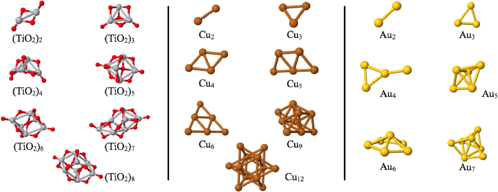
In addition to the properties of light elements from the first and second row of the periodic table, we also investigated the performance of RI-LVL for a few representative heavier elements, namely copper, gold and titanium dioxide. The cluster geometries used for this test are displayed in figure 9.

Figure 9. The clusters we used to benchmark the performance of RI-LVL for heavy elements. The geometries of all clusters can be found in the supporting information. The gold [63] and titanium-dioxide clusters [64] are the results from basin hopping and genetic algorithm based structure optimizations. The copper clusters [65] are cut out from bulk geometries.
Download figure:
Standard image High-resolution imageFigure 10 shows the RMSD and maximum absolute error per atom for titanium dioxide, copper and gold clusters. For the heavy elements we used either tier 3 (titanium, oxygen and gold) or tier 4 (copper) basis sets to demonstrate the applicability of our new method to a typical RPA-calculation setup. We know from the previous results that light elements like oxygen need an enhanced auxiliary basis set for an accurate treatment with RI-LVL. Therefore, we constructed an enhanced auxiliary basis set with an additional g-function (z = 1) for oxygen in titanium dioxide. For the explicit three-center integrals of RI-V, dense multicenter integration grids are needed for heavy elements. We note that the integrals are two-center in RI-LVL and can be carried out using Talman's method, therefore significantly lighter integration grids are sufficient for our RI-LVL implementation than for RI-V. With very tight integration settings (see appendix


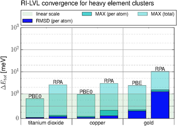
Figure 10. Total energy error of the RI-LVL RPA@PBE0 calculations for TiO2 (2–8 units), Cu (2–6,9 and 12 atoms) and Au clusters(2–7 atoms). The reference point is the RI-V calculation with the standard tier3/4 basis sets. In the TiO2 case the oxygen atoms had an OBS+ with a g-function for the RI-LVL calculation. See SI for details.
Download figure:
Standard image High-resolution imageTo substantiate this observation, we computed the systems again with a g-function in the OBS+ and otherwise identical parameters. The results are shown in table 9.
Table 9. For RI-V and RI-LVL, we show the RPA@PBE0 total energy change (RMSD) of the clusters shown in figure 9 when adding a g-function (z = 6) to the OBS of the elements Ti, Cu, and Au. For all titanium dioxide test cases, we used an OBS+ with an additional g-function on oxygen, i.e., the third column only reflects the RMSD change due to the addition of a g-function to the OBS of Ti. See text for further details about the computational settings.
| RPA-RMSD per atom | RMSD per | |
|---|---|---|
| OBS+ with g[z = 6] versus standard OBS | atom (meV) | |
| Gold | RI-V | 0.438 |
| OBS: tier 3 | RI-LVL | 0.187 |
| Copper | RI-V | 0.193 |
| OBS: tier 4 | RI-LVL | 0.043 |
| Titanium dioxide | RI-V | 0.101 |
| OBS: tier | RI-LVL | 0.022 |

Enhancing the RI-LVL calculations with additional auxiliary basis functions on the heavy elements changes the results only slightly. The RI-V calculations on the other hand show a larger, but overall still insignificant susceptibility to the additional functions in the . For example the RMSD changes by 0.44 meV for gold when computed with RI-V, while RI-LVL only exhibits a change of 0.19 meV.

From the presented RMSD and maximum errors (figure 10) we can see that RI-LVL is very accurate for heavy elements and can reproduce the RI-V results with no significant error. The deviation for the error per atom is consistently below 1.5 meV and even the total error is a few meV at most for large basis sets. We have additionally verified that these conclusions also hold for smaller FHI-aims tier1 basis sets as the OBS for Ti, Cu, and Au, with maximum overall errors between RI-LVL and RI-V for RPA of 3 meV (Au7) and errors for the PBE0 hybrid functional consistently below 1 meV. The good performance for all three elements shows that the RI-LVL has no problems dealing with d- and f-electrons.
4. Computational scaling analysis
In addition to the accuracy of the localized RI, we also investigated the scaling with system size, i.e. the number of atoms, both in terms of memory consumption and the required computational time. To obtain a superior scaling with our localized variant, specialized routines are required that operate on the resulting sparse tensors instead of on the full three-function tensor. At present, such routines exist for the evaluation of the Fock matrix within FHI-aims. This implementation is discussed in detail in a separate publication [34]. In particular this implementation employs integral screening as used in standard quantum chemistry linear scaling exchange algorithms based on density matrix screening [55, 69].
Figure 11 shows the scaling of the RI-LVL (using sparsity and screening) in comparison to RI-V for the HF level of theory for extended polyalanine chains. One of them, namely Alanine-8 (Ala8) is depicted in figure 11(b). All calculations were performed using the tier 2 basis sets [16] and tight integrations settings (see table 1 in [70] for details). The auxiliary basis in RI-LVL was enhanced with one extra g-function (z = 6).

Figure 11. Scaling analysis of self-consistent Hartree–Fock calculations for fully extended oligoalanine chains. The figures show the RI-V implementation and the RI-LVL version that uses sparsity as well as integral screening. All calculations were performed using 180 CPU cores of an Infiniband-connected Intel cluster with Intel Xeon X5650 Westmere hexa-core processors (2.66 GHz, 12 cores per node). As computational settings we used the tight defaults settings and the tier 2 basis set. For the RI-LVL calculations we furthermore added one more radial g-function with z = 6 for the construction of the auxiliary basis.
Download figure:
Standard image High-resolution imageFigure 11(a) shows the total time required for the self-consistent HF calculation, as well as the portion that is spent on the Fock matrix evaluations. In small systems, the screened RI-LVL runs slower compared to simple BLAS3 dense matrix multiplications used in RI-V. The break-even point occurs at about 70 atoms. For RI-LVL, in contrast to RI-V, the Fock matrix evaluation is the single dominant contribution to the total time, regardless of the system size. This shows that the localized scheme significantly speeds up the construction of the auxiliary basis.
Figure 11(c) shows how the memory consumption for RI-V and RI-LVL scales with system size. While RI-LVL has a large constant offset, it scales linearly and breaks even at only 50 atoms. The favorable memory scaling is due to the fact that we no longer need to store the complete three-center integrals . Each core p has a peak memory requirement Mp. For both methods an increase in the spread between minimal () and maximal () memory consumption per core can be observed with increasing system size. This is a consequence of a load-balancing algorithm [34]. Figure 11(d) shows the difference in the total energy per atom between RI-V and RI-LVL. The error per atom is insignificant and does not increase with system size, but instead levels out at a very low value.


Finally, we extrapolated the scaling of the computational time for the algorithm with system size by analyzing the scaling of its dominant step, namely the evaluation of the exchange matrix. In figure 12 we present the scaling of the time necessary for the exchange matrix evaluation as a function of the system size approximated by the second SCF-iteration. Shown are the results for RI-V using the standard auxiliary basis and 180 cores (to accommodate the memory needs of the largest system tested) and for RI-LVL with the enhanced auxiliary basis on 24 cores. Our localized RI exhibits a superior scaling (linear versus cubic) and despite using significantly fewer cores, the break-even point occurs at around 110 atoms.

Figure 12. Time for the Fock matrix evaluation in the second SCF step of fully extended oligoalanine chains of increasing length. In the graph, we compare data for the RI-V implementation and for the RI-LVL version that uses sparsity as well as integral screening. The RI-V based calculations were performed in parallel on 180 CPU cores, while the RI-LVL based calculations were performed using 24 CPU cores (same hardware as described in caption of figure 11). As computational settings we used the tight defaults settings and the tier 2 basis set. For the RI-LVL calculations we furthermore added one more radial g-function with z = 6 for the construction of the auxiliary basis.
Download figure:
Standard image High-resolution image5. Conclusion and outlook
In this work, we present a way to improve the scaling of the RI technique with the number of atoms by restricting the expansion to a subset of the auxiliary basis functions. 'RI-LVL' only includes auxiliary basis functions which are located at one of the two atoms where the basis functions forming the product are centered. Importantly, the Coulomb metric of RI-V is retained.
We show for HF, DFT-PBE0, MP2, and RPA that the error of the RI-LVL approach can be controlled in a systematic way by enhancing the set of orbital basis functions, upon which the auxiliary basis for RI is based, with specific, structure- and method-independent additional radial functions before the auxiliary basis set itself is built. For light elements, by using functions up to angular momentum channel g we were able to reduce the RMSD of the total energy (compared to an RI-V calculation with the pure basis set) below 1 meV for the S22 test set. Even for sub-meV total energy accuracy, we found that a single g function in the OBS+ is sufficient. For heavy elements, no enhancement of the orbital basis set for the purpose of constructing the RI auxiliary basis set is needed. We also showed that RI-LVL has a similar performance for reaction barrier heights and atomization energies in molecular systems. The RI-LVL method also requires less dense integration grids for the same accuracy as RI-V for heavy elements with very large basis sets.

The RI-LVL method together with these auxiliary basis sets paves the way towards low-memory, linear-scaling implementations of HF exchange, MP2, RPA and even higher-level methods.
Acknowledgments
This work was partially supported by the DFG Cluster of Excellence UNICAT. Patrick Rinke acknowledges funding from the Academy of Finland through its Centres of Excellence Program (#251748).
Appendix A: Employed basis sets
The FHI-aims code includes NAO basis sets consisting of successive 'tiers' or levels of groups of radial functions. The basis sets include the free-atom solutions for occupied orbitals of the given element and hydrogen-like functions. In some cases also functions from the free ion are used to complement the basis set. The tier basis sets used in this paper are listed in table 10. The table only lists the radial functions, which are then multiplied with all spherical harmonics for their given angular momentum.
Appendix B: The effects of augmenting the orbital basis set
As shown above, adding a single hydrogen-like function with angular momentum g to the pool of functions used to construct the auxiliary basis set in RI-LVL suffices to recover the accuracy of the RI-V. To give a specific example of the number and type of radial functions recovered at each step of the construction procedure outlined in figure 1, table 12 summarizes the pertinent radial functions in the orbital and auxiliary basis sets of the C atom, using the GTO cc-pVTZ and the NAO tier 2 basis sets as examples. All specifics of the radial functions up to tier 2 are summarized in table 10. As it can be seen from the table, adding a single g-function to the construction procedure yields a large set of additional auxiliary basis functions.
Appendix C: Integration parameters for heavy element tests
FHI-aims uses an atom-centered grid for computing most integrals [16, 54]. The grid is composed of radial 'shells' [71] (see also equation (18) in [16] and the appendix in [61]) and each shell is populated with a given number of angular integration points that form a Lebedev grid [72–75]. The key controlling parameters for the accuracy of the integration routines are the number of radial shells and the number of angular grid points as a function of the distance to the center. For our investigation of heavy elements, we use dense integration grids, because our reference point, the RI-V, is sensitive to the quality of the grid. The details are listed in table 11. For the sake of consistency we decided to use the same integration settings also in RI-LVL. In a production calculation the settings can be reduced significantly, because RI-LVL does not use the atom-centered grid for the four-center integral evaluation and the normal DFT part has much lower demands on the grid settings.
Table 10. Numerical parameters of the radial functions defining the NAO basis sets employed in FHI-aims as described in detail in [16]. Basis sets consist of a minimal free-atom like set of radial functions, and additional 'tiers' (levels) of radial functions as determined by an automated basis set construction procedure. The label '' denotes a hydrogen-like function with principal quantum number n, angular momentum l and the effective charge z. The label '' denotes free-ion solutions with the given ion charge z and the quantum numbers n and l. Each tier includes the functions from all preceding tiers.


| H | C | N | O | Ti | Cu | Au | |
|---|---|---|---|---|---|---|---|
| Minimal | 1s | [He] + 2s, 2p | [He] + 2s, 2p | [He] + 2s, 2p | [Ar] + 4s, 3d | [Ar] + 4s, 3d | [Xe] + 6s, 5d, 4f |
| Tier 1 | H(2s, 2.1) | H(2p, 1.7) | H(2p, 1.8) | H(2p, 1.8) | H(4f, 8.0) | Cu2+(4p) | Au2+(6p) |
| H(2p, 3.5) | H(3d, 6.0) | H(3d, 6.8) | H(3d, 7.6) | H(3d, 2.7) | H(4f, 7.4) | H(4f, 7.4) | |
| H(2s, 4.9) | H(3s, 5.8) | H(3s, 6.4) | Ti2+(4p) | H(3s, 2.6) | Au2+(6s) | ||
| H(5g, 11.6) | H(3d, 5.0) | H(5g, 10.0) | |||||
| Ti2+(4s) | H(5g, 10.4) | H(6h, 12.8) | |||||
| H(3d, 2.5) | |||||||
| Tier 2 | H(1s, 0.8) | H(4f, 9.8) | H(4f, 10.8) | H(4f, 11.6) | H(3d, 4.4) | H(4p, 5.8) | H(5f, 14.8) |
| H(2p, 3.7) | H(3p, 5.2) | H(3p, 5.8) | H(3p, 6.2) | H(6h, 16.0) | H(3d, 2.7) | H(4d, 3.9) | |
| H(2s, 1.2) | H(3s, 4.3) | H(1s, 0.8) | H(3d, 5.6) | H(4f, 9.4) | H(6h, 15.2) | H(3p, 3.3) | |
| H(3d, 7.0) | H(5g, 14.4) | H(5g, 16.0) | H(5g, 17.6) | H(4p, 4.5) | H(5s, 10.8) | H(1s, 0.5) | |
| H(3d, 6.2) | H(3d, 4.9) | H(1s, 0.8) | H(1s, 0.5) | H(4f, 16.0) | H(5g, 16.4) | ||
| H(6h, 13.6) | |||||||
| Tier 3 | H(4f, 11.2) | H(2p, 5.6) | H(3s, 16.0) | (2p) | H(4d, 6.4) | H(4d, 6.0) | H(4f, 5.2) |
| H(3p, 4.8) | H(2s, 1.4) | (2p) | H(4f, 10.8) | H(4f, 10.0) | H(3p, 2.4) | H(4d, 5.0) | |
| H(4d, 9.0) | H(3d, 4.9) | H(3d, 6.6) | H(4d, 4.7) | H(5g, 12.0) | H(4f, 6.4) | H(5g, 8.0) | |
| H(3 s, 3.2) | H(4f, 11.2) | H(4f, 11.6) | H(2s, 6.8) | H(2p, 1.7) | H(3s, 6.8) | H(5p, 8.2) | |
| H(6h, 16.4) | H(5g, 11.2) | H(6d, 12.4) | |||||
| H(4s, 3.8) | H(6s, 14.8) | ||||||
| Tier 4 | H(2p, 2.1) | H(2p, 4.5) | H(3p, 5.0) | H(4p, 7.0) | |||
| H(5g, 16.4) | H(2s, 2.4) | H(3s, 3.3) | H(4s, 4.0) | ||||
| H(4d, 13.2) | H(5g, 14.4) | H(5g, 15.6) | H(6h, 14.0) | ||||
| H(3s, 13.6) | H(4d, 14.4) | H(4f, 17.6) | H(4d, 8.6) | ||||
| H(4f, 17.6) | H(4f, 16.8) | H(4d, 14.0) | H(5f, 15.2) |


Table 11. Highly converged integration settings for the different atoms. Nr denotes the final number of radial shells. Nrbase is the initial number of shells before the enhancement factor rmult, also known as the radial multiplier, is applied and router is the outermost radius of the base integration grid. (see appendix of [61] for details) Nang is the number of grid points on an integration shell.
| Quantity | Au | Cu | Ti | O |
|---|---|---|---|---|
| Nr | 443 | 323 | 293 | 221 |
| Nrbase | 73 | 53 | 48 | 36 |
| rmult | 6 | 6 | 6 | 6 |
| router | 7 Å | 7 Å | 7 Å | 7 Å |
| 110 | 110 | 110 | 110 | |
| 974 | 974 | 974 | 974 |


Table 12. The size of the auxiliary basis set for a carbon atom with a standard and augmented auxiliary basis for both the cc-pVTZ and tier 2 basis sets in FHI-aims, corresponding to the steps outlined in figure 1. In this table, the notation indicates the inclusion of four different s-type radial functions. The expression 'number of radial functions' refers to the number of distinct radial functions used in the construction of orbital or auxiliary basis sets, whereas the expression 'number of basis functions' counts the total number of basis functions in the sets or . Thus, the 'number of basis functions' also accounts for the different angular momentum functions Ylm included in their definition in equation (8).


| Standard orbital basis | Augmented orbital basis | |||
|---|---|---|---|---|
| cc-pVTZ | Tier2 | cc-pVTZ | Tier2 | |
| Number of basis functions in orbital basis | 30 | 39 | 30 | 39 |
| Pool of radial functions uskl for auxiliary basis construction | , , , | , , , , | , , , , | , , , , |
| Number of onsite radial products | 111 | 150 | 150 | 198 |
| Number of onsite radial functions in auxiliary basis after Gram-Schmidt orthonormalization | 43 | 50 | 65 | 70 |
| Types of radial functions in the auxiliary basis | , , , , , , | , , , , , , , , | , , , , , , , , | , , , , , , , , |
| Final number of basis functions in auxiliary basis | 225 | 310 | 445 | 518 |


