


Abstract
We investigate, within Floquet theory, topological phases in the out-of-equilibrium system that consists of fermions in a circularly shaken honeycomb optical lattice. We concentrate on the intermediate regime, in which the shaking frequency is of the same order of magnitude as the band width, such that adjacent Floquet bands start to overlap, creating a hierarchy of band inversions. It is shown that two-phonon resonances provide a topological phase that can be described within the Bernevig–Hughes–Zhang model of HgTe quantum wells. This allows for an understanding of out-of-equilibrium topological phases in terms of simple band inversions, similar to equilibrium systems.
Export citation and abstract BibTeX RIS

Content from this work may be used under the terms of the Creative Commons Attribution 3.0 licence. Any further distribution of this work must maintain attribution to the author(s) and the title of the work, journal citation and DOI.
1. Introduction
Ultracold atom setups provide experimentalists with a highly tunable framework that can be used to simulate quantum systems (Lewenstein et al 2007, Bloch et al 2008). For example, one can create quasi-periodic one-dimensional systems (Amico et al 2005), realise p-band condensates (Wirth et al 2011, Ölschläger et al 2013), or even do atomtronics (Seaman et al 2007), which aims at simulating electronic circuits. Due to this great flexibility, the recent realisation of topological states in condensed-matter systems (König et al 2007, Hasan and Kane 2010, Qi and Zhang 2010) has sparked a flurry of activities in the field of cold atoms, aiming at reproducing, engineering, and manipulating these fascinating quantum states in traps (Roncaglia et al 2011, Corman et al 2014, Burrello et al 2015) and in optical lattices (Hemmerich and Morais Smith 2007, Aidelsburger et al 2013, Miyake et al 2013, Jotzu et al 2014, Aidelsburger et al 2015, Chomaz et al 2015).
Topological fermionic systems exhibit protected conducting states at the boundary, while the bulk of the material remains insulating. In cold atoms, quantised transverse density currents play the role of the quantised charge currents, since we deal with neutral atoms in selected hyperfine states, instead of spin-full electrons. Similarly, the pair of atomic hyperfine states yields a spin-1/2 structure that allows for the analogue of quantised spin currents obtained in condensed-matter systems. The conductivity at the boundary is given by a topological invariant, which is quantised and stable against perturbations.
There are a variety of fermionic topological states known by now, and in certain cases they are well described by the ten-fold classification (Ryu et al 2010), which defines a topological invariant according to the symmetries and dimensionality of the system. Although well established, the ten-fold classification neglects several effects. First, it only describes systems of free fermions. Although this includes interacting systems which have a free fermionic quasiparticle description, like topological superconductors, it cannot describe strongly correlated topological phases like fractional quantum Hall systems (Tsui 1982, Laughlin 1983). It also cannot describe other interaction induced phenomena like the quantum anomalous Hall effect (Nandkishore and Levitov 2010, Jung et al 2011), or a quantum valley Hall effect (Marino et al 2015). Second, it does not consider the crystal symmetry of the lattice, which may give rise to crystalline topological insulators (TI's), and even more general behaviour (Slager et al 2013). Last, but not least, it does not take into account out-of-equilibrium systems.
The case of TI's under the influence of a time-periodic perturbation, the so-called Floquet TI's (FTI's) (Inoue and Tanaka 2010, Gu et al 2011, Kitagawa et al 2011, Lindner et al 2011, Ezawa 2013, Fregoso et al 2013, Rudner et al 2013, Wang et al 2013, Fregoso et al 2014, Gomez-Leon et al 2014, Perez-Piskunow et al 2014, Quelle and Morais Smith 2014, Kundu et al 2014, Usaj et al 2014, Carpentier et al 2015), has, until now, been considered in three unequal regimes. Firstly the so-called quasi-equilibrium regime, where  here J is the hopping parameter, which is roughly the bandwidth of the relevant set of bands, ω the driving frequency, and Δ the gap between the next set of bands. In this case, the system constituents cannot follow the perturbation, and the system remains at quasi-equilibrium with simply renormalised lattice parameters. It is the regime that has been most studied (Eckardt et al 2005, Zenesini et al 2009, Koghee et al 2012, Struck et al 2013, Goldman and Dalibard 2014). Secondly, the regime where
  This regime is starting to attract interest in optical lattices (Parker et al 2013, Zheng and Zhai 2014, Zheng et al 2014), but it has been unexplored in the context of condensed matter. Thirdly, the regime where
  , and where the equilibrium topological classification breaks down. It is this regime where most of the work on FTI's in condensed matter has taken place, and these kind of systems have even been simulated in twisted photonic waveguides (Rechtsman et al 2013), where the third spatial dimension takes the role of time. There have been attempts to define Chern-type topological invariants valid for every frequency range (Lindner et al 2011, Rudner et al 2013, Carpentier et al 2015), and it is known that these invariants reduce to the equilibrium ones in the first regime. The transition between the first and third regime has been investigated theoretically in (Kundu et al 2014) for graphene irradiated by circularly polarised light, and in (Gómez-León and Platero 2013) for the case of a periodically driven dimer chain. However, for the case of ultracold atoms, this regime has so far been overlooked.
Here, we show that for circularly shaken honeycomb optical lattices the transition between the first and third regime can be understood in terms of band inversion. These band inversions occur because, with decreasing frequency, the different Floquet bands start to overlap, causing a band inversion. Because the circular shaking induces phonon resonances, these band inversions cause the opening of gaps in the system that generally host topological edge states. The polarisation of the shaking breaks time-reversal symmetry, such that the resulting FTI is in class A of the ten-fold classification. This class also contains the quantum Hall systems, and its distinguishing feature is a quantised edge conductance, as given by the Chern number. It should be noted that this topological phase is achieved in the absence of a magnetic field, so although there are conducting edge states, no Landau levels are present in the system. It has recently been shown that one-phonon resonances create an additional topological gap in the spectrum at non-zero energy, whereas two-phonon resonances destroy the topological nature of the zero-energy gap by creating counter-propagating edge states (Quelle and Morais Smith 2014). Here, we derive an effective continuum model from the out-of-equilibrium lattice model, and show that, in the vicinity of the band inversion occurring for the two-phonon resonances, it turns out to be described by the Bernevig–Hughes–Zhang (BHZ) model (Bernevig et al 2006). Additionally, we demonstrate the validity of this model by comparing our results with a numerical solution of the full problem. In this way, our results describe the transition between the quasi-equilibrium and the resonant regimes of the shaken system, by modelling the appearance of phonon resonances in the latter regime in terms of band inversions. This provides a link between non-equilibrium and equilibrium topological states of matter. Finally, we discuss a possible experimental observation in shaken honeycomb optical lattices loaded with ultracold fermions, as well as in the recently realised honeycomb superlattices of CdSe nanocrystals (Boneschanscher 2014, Kalesaki et al 2014).
2. The Hamiltonian in co-moving coordinates
Consider an optical lattice that is shaken in time. The deviation of the lattice from its equilibrium position is denoted by  by assumption
  for some period T. To find the Hamiltonian in co-moving coordinates, we consider the Poincaré–Cartan form

along the trajectory of a system in phase space. We change coordinates to co-moving coordinates  ,
,  , such that
  and
and 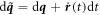 , where
  is the time derivative of
  . The Poincaré–Cartan form can thus be rewritten as

We immediately read off the Hamiltonian in co-moving coordinates: 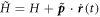 . The extra term encodes the pseudoforces seen because the co-moving frame is not inertial. For a shaken optical lattice, the Hamiltonian reads

where the potential determines the lattice, which we take to be honeycomb.
In the co-moving frame  and
and  , equation (3) becomes
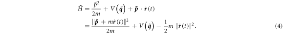
For circular shaking,  which means
  is constant in time and can be ignored by shifting the energy. The circular shaking thus induces a rotating vector potential
  , which has constant magnitude
  . This is equivalent to the Hamiltonian for a system irradiated by circularly polarised light, where
  for an electric field E.
3. Floquet theory
The Hamiltonian in equation (4) is periodic in time, so according to Floquet theory (Sambe 1973, Hemmerich 2010), the time-dependent Schrödinger equation has quasi-periodic solutions 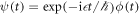 , where ϕ is a periodic function in time and thus a solution of
  Here, the Floquet Hamiltonian is defined as
  If H acts on the Hilbert space
  and
and  is the Hilbert space of T-periodic functions, then HF acts on
  . The space
  is spanned by the functions
  , and has inner product
  . With respect to the states
  we can write HF as a block matrix with elements

Here, we defined  to be the Fourier modes of the original Hamiltonian H.
4. Model
We apply the Floquet formalism to spinless fermions in a circularly shaken honeycomb lattice, with shaking radius r0, and frequency ω. We work in the co-moving reference frame, where the Hamiltonian has the form in equation (4). To facilitate our analysis, we use the tight-binding approximation, as done for graphene (Castro Neto et al 2009). In second quantisation, the result is the Bloch Hamiltonian, except that one has to account for the vector potential according to the Peierls substitution, 

Here,  is the NN hopping amplitude, and our convention for the NN hopping vectors
  is
is  and
and  where a is the NN distance. Consequently, one obtains, via equation (5), the matrices
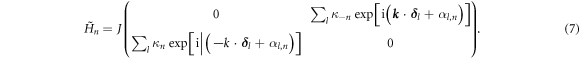
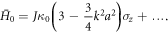
In equation (7),  where Jn is the Bessel function of the nth kind, and
 ![${\alpha }_{l,n}:= n{\rm{Arg}}[{{\boldsymbol{\delta }}}_{l}]+n\pi /2$](https://content.cld.iop.org/journals/1367-2630/18/1/015006/revision1/njpaa0cf2ieqn38.gif) , where
, where  gives the angle of a vector with the x-axis. Using equation (7), we obtain
  as an infinite block matrix
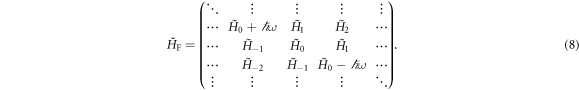
If the spectrum around an energy  is desired, it can be computed by truncating the right-hand side of equation (8) around
  By tuning the shaking frequency ω, one may reach certain regimes where
  exhibits topological edge states. In the large-frequency limit,
  , the Floquet bands are well separated, but one finds a hierarchy of band crossings upon decrease of ω, when
  . These band-crossings create additional, possibly topological gaps in the spectrum. In the following, we focus on the band crossing in the vicinity of k = 0 and
  , appearing in the interesting regime:
  . In figure 1, the spectrum of
  is plotted for
  . In figure 1(a), we have made the n = 0 Floquet band translucent to draw attention to the impending band inversion. The bottom of the n = 1 valence band (on top) and the top of the n = −1 conduction band (below) are visible with a gap between them. In figure 1(b), the n = 1 and n = −1 Floquet bands have been made translucent to draw attention to the n = 0 Floquet band, which hosts topological edge states at the Dirac points. It should be noted that the bottom half of figure 1(b) is identical to the top half of figure 1(a). This is because the spectrum is periodic in
  , so the n = 0 valence band in figure 1(b) is identical to the n = 1 valence band in figure 1(a). The full spectrum can be obtained by superimposing figures 1(a) and (b), since the bands n = ±1 and n = 0 are the only ones visible in the first two periods of the spectrum. As ω is lowered, the valence band (on top in figure 1(a)) descends and the conduction band (at the bottom of figure 1(a)) ascends; a band inversion takes place at
  , and due to the radiation, the gap reopens after the bands invert (figure 2(a)). An extra pair of edge states now crosses the gap where the band inversion took place, as is highlighted in figure 2(b), where we show a zoom in on a narrow energy window. It should be noted that the edge states at the Dirac points (figure 1(b)) are still present after the band inversion, and the edge states at k = 0, which correspond to the two-phonon resonance, are counter-propagating with respect to them. (In figure 2, the edge states at the Dirac points have been made translucent at
  to avoid confusion. They are depicted at
  , which are equivalent to
  due to the periodicity of the Floquet spectrum; in these gaps, instead, the two-phonon resonance states have been made translucent.) The appearance of new edge states at k = 0 removes the topological protection of the edge states in the
  gap (Quelle and Morais Smith 2014). This can be seen by considering the topological winding number for the system (Rudner et al 2013). Because the two states counter-propagate, they contribute to this winding number with opposite sign, as can be checked by an explicit calculation. Furthermore, this lack of topological protection becomes evident in a lattice with armchair termination, where the zero-phonon and two-phonon resonances both occur at k = 0. Indeed, in this case they gap out because of hybridisation, which could not have occurred if the states were topologically protected. In contrast, if only the edge state at the Dirac points is present, changing to the armchair termination does not gap it out. Finally, it is possible to create a domain wall where the orientation of the circularly polarised light changes. This domain wall creates a boundary where the topological phase of the material changes, which causes the presence of protected states localised at the domain wall. If the counter-propagating states at k = 0 and the Dirac points are present, no gapless states are present at such a domain wall, which indicates that the gap must be trivial. Physically, the gapless states at the domain wall can hybridise because they can hop across the phase boundary, which causes them to gap out (Quelle et al 2014). These considerations show that the appearance of the two-phonon resonance indeed makes the
  gap trivial. The situation can be reversed by applying a staggered sublattice potential: this will destroy the zero-phonon resonance at the Dirac points, but leave the two-phonon resonance untouched. In this case, the appearance of the two-phonon resonance changes the gap at
  from topologically trivial to non-trivial.

Figure 1. (a) The spectrum of the Floquet Hamiltonian  is shown. Plots were made for a ribbon geometry with zigzag edges, and k denotes the Bloch momentum along the length of the ribbon. Two periods of the spectrum of
  are shown for
  and
and  The relevant feature is the impending gap closure at
  and k = 0, when the Floquet bands n = 1 and n = −1 overlap. To highlight this, we have made all bands, except for n = 1 and n = −1, translucent. Red and blue represent different edges. The y-axis is labelled in terms of
  . (b) The same spectrum as in (a) is shown, but now all bands except for n = 0 have been made translucent. This draws attention to the edge states at the Dirac points in the
  gap. The one-phonon resonance at
  is also visible in this figure, because it is caused by an overlap between the n = 0 and n = ±1 bands.
Download figure:
Standard image High-resolution image
Figure 2. (a) Same as in figure 1, but for  . The relevant feature is the band inversion at
  and k = 0, where the Floquet bands n = 1 and n = −1 overlap, creating a gap with topologically protected edge states. To highlight this, we have made all bands, except for n = 1 and n = −1, translucent. (b) A zoom in on the band crossing from (a) is provided to make the details of the gap visible.
Download figure:
Standard image High-resolution image
5. Low-energy effective theory
To write down an effective theory that allows us to characterise the band crossing, the gap and the dispersion of the edge states, we extract the relevant energy bands from  . This is done by diagonalising
  , and for simplicity we keep terms up to second order in
  . We define the unitary transformation

and consider the transformed Hamiltonian

where  by construction. From equations (7) to (9), one finds the identity
It follows that for  and
and  the
the  element of the matrix
  and the
  element of
  are much smaller than all the other energy scales in the problem. They are the zeroth-order energies of the two bands near the band crossing shown in figures 1 and 2. This leads us to define a second unitary transformation V that is characterised by the matrix elements
  and that permutes the basis vectors in such a way that the
  elements of the 2 × 2 matrices along the diagonal of
  are interchanged with the
  elements diagonally above. Here,
 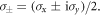 With respect to this basis, the Floquet Hamiltonian
  reads
reads
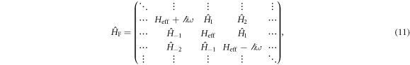
where the  are more complicated matrices obtained by interchanging elements of the
  , which do not need to be defined here. It follows that

where the superscripts denote a specific element of the corresponding matrix. Due to its periodic structure, the matrix in equation (11) has only two eigenvalues that repeat with periodicity  These eigenvalues correspond to an effective 2 × 2 Hamiltonian that can be found through a series expansion detailed in (Goldman and Dalibard 2014). This expansion is in orders of
  and the size of the
  , which is
  in this specific case. The lowest order term is precisely
  , and the first correction is
 ![$[{\hat{H}}_{-1},{\hat{H}}_{1}]/\omega $](https://content.cld.iop.org/journals/1367-2630/18/1/015006/revision1/njpaa0cf2ieqn91.gif) . All higher-order corrections have similar expressions in terms of commutators containing the
. All higher-order corrections have similar expressions in terms of commutators containing the  and powers of
  . Because the
  contain progressively higher orders of
  this series expansion can be truncated when the matrix elements of
  are small compared to ω, and
  . For example,
 ![$[{\hat{H}}_{-1},{\hat{H}}_{1}]$](https://content.cld.iop.org/journals/1367-2630/18/1/015006/revision1/njpaa0cf2ieqn98.gif) is of the same order as
is of the same order as  , so
, so ![$[{\hat{H}}_{-1},{\hat{H}}_{1}]/\omega $](https://content.cld.iop.org/journals/1367-2630/18/1/015006/revision1/njpaa0cf2ieqn100.gif) is supressed by an extra factor of
is supressed by an extra factor of  when the elements of
  are small. Around the two-phonon resonance, with the values of
  used to generate figures 1 and 2, all higher-order terms can be dropped from the expansion, and
  is the desired effective Hamiltonian. This can be seen from a comparison with numerical calculations, which shows that equation (12) is sufficient to accurately describe both the gap size and the presence of the topological states; see figure 2(b) for example. For small ω and/or large shaking velocities
  , the higher-order terms in the series do not decay, and they cannot be dropped from the expansion. The deviations caused by these extra terms have been investigated numerically in (Perez-Piskunow et al 2015), which describes the irradiated condensed matter analogue of this system. This system is equivalent to ours, if one sends
  , where
  is the magnitude of the vector potential describing the applied radiation. They conclude that increasing the radiation amplitude E can lead to phase transitions without additional band inversions, as the off-diagonal blocks become sizeable. This behaviour would also occur in the shaken optical lattice under an increase of
  from the values used to generate figures 1 and 2.
Similarly, higher-phonon resonances occur at low values of ω and hence require the inclusion of higher-order terms in the effective Hamiltonian. Our method can also be used to model the one-phonon resonance, but the form of the effective Hamiltonian will be different, as can be seen from the different topological properties connected with this resonance. More details on the one-phonon resonance are given in the appendix. Using the definition of  , one obtains
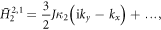
and thus the BHZ Hamiltonian (Bernevig et al 2006)

where

These expressions are correct up to order  , and agree with the ones derived by Kundu et al upon replacing
  by
by  . The presence of the Bessel function of the second kind, J2, through
  in equation (14), shows that the opening of a gap at the band inversion is a second-order phonon process. It should be noted that for the NN-hopping
  , one finds that A in equation (14) acquires an additional minus sign, but the spectrum remains unaffected. Finally, honeycomb optical lattices with a slight deformation of the unit cell that breaks the three fold symmetry at each lattice site have recently been experimentally realised (Tarruell et al 2012). Such an anisotropy in the unit cell will change the effective Hamiltonian since the bond length a enters it through
  , causing
  to become direction dependent. For small anisotropies, the results discussed above should still hold, except that the precise values of
  where the two-phonon resonance occurs will depend on the renormalised
  parameters, and the gap size will now become direction dependent.
6. Edge states and gap size
From the effective Hamiltonian in equation (13), and following (Qi and Zhang 2010), one can derive an explicit solution for the edge state in the infinite half-plane. Using perturbation theory to linear order in k, the edge states then disperse as
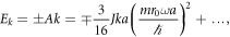
i.e. the edge states have a velocity quadratic in the frequency ω.
From  , an expression for the gap size Δ can also be derived, and one obtains

Substituting the parameter values  and
and  into equation (15) yields a gap size
  , which is in good agreement with the numerical results shown in figure 2(b).
7. Conclusion
In conclusion, we have investigated fermions in a circularly shaken honeycomb optical lattice in the intermediate regime, where the shaking frequency is on the order of the bandwidth  . In this particular regime, the system is characterised by a substantial overlap between the Floquet side bands, and a series of band inversions can be created that generally host topological edge states. We have concentrated on the crossing associated with two-phonon resonances, at
  , and we have shown that the relevant effective continuum model is just the BHZ model for HgTe quantum wells. This allows for an understanding of the transition between the quasi-equilibrium regime and the resonant regime in terms of well-studied effective models, and especially in terms of band inversion, now between adjacent Floquet bands.
Considering that the model Hamiltonian also describes a honeycomb lattice irradiated with circularly polarised light, the question remains whether the discussed effects can be observed in condensed matter. In this case, the phonon resonances become photon resonances, but the prior calculations remain valid, simply by replacing  by
by  . A natural candidate would be graphene, but the relevant hopping parameter
  and the NN bond length
  Å in graphene would require unphysically large frequencies beyond the THz regime, and a very high field strength of
  V m−1. A more promising candidate is a self-assembled honeycomb lattice of CdSe nanocrystals (Boneschanscher 2014, Kalesaki et al 2014), which hosts an s-band exhibiting a dispersion similar to that of graphene. The hopping parameter in these artificial structures depends on the diameter and the contact area of the nanocrystals. A hopping parameter J = 25 meV, that is roughly two orders of magnitude smaller than that in graphene, has been theoretically predicted for nanocrystals with a diameter of 3.4 nm (Kalesaki et al 2014). By using light with
  m−1 and
  meV, a gap of 1.5 meV is obtained for these parameters, which is
  of the hopping J. In Wang et al (2013), the Dirac states at the surface of a 3D topological insulator are irradiated by circularly polarised light, and the resulting photon resonance gaps are detected using ARPES. Although thermal excitation of the Dirac electrons is observed, it is possible to measure the Floquet spectrum before the states have been excited away from the bands. This, together with the predicted bandgap, implies that the two-photon resonance should be observable in the recently synthesised artificial superlattices of CdSe nanocrystals (Boneschanscher 2014, Kalesaki et al 2014), or in predicted similar structures (Beugeling et al 2015).
It would be much more natural to attempt to realise the Hamiltonian in equation (13) through the use of optical lattices. Honeycomb lattices have been manufactured in the past (Soltan-Panahi et al 2011), and they are more promising for two reasons. The first reason for this is the much larger lattice constant, compared to condensed matter systems: since the vector potential enters the Hamiltonian in the combination  this allows for smaller vector potentials. The second reason is that the circular shaking described here creates a vector potential of the form
  , as opposed to
  , so that increasing the frequency actually increases the vector potential, rather than suppressing it. In graphene, for example, the required frequencies suppress the vector potential too strongly, resulting in the necessity of unphysically large electric fields. In contrast, taking a honeycomb optical lattice with NN hopping J and recoil energy
  , we can rewrite
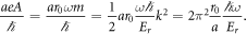
To obtain the bandgap derived in the previous section would require shaking by a frequency  , at a radius
  . For potassium atoms loaded in an optical lattice with wavelength k = 1064 nm, which corresponds to
  , the shaking would be at several kHz, with a radius of several tens of nm, which means several percent of the lattice constant. Since possible shaking amplitudes range from this regime (Jotzu et al 2014) up to several times the optical wavelength (Struck et al 2011), these parameters are easily achievable experimentally. This suggests that honeycomb optical lattices are a very promising candidate for realising the topological states discussed here. The richness of shaking protocols, which are a hallmark of optical lattices, together with these encouraging results, promise that the up-and-coming field of atomtronics could be a prime candidate for the experimental investigation of FTI's.
Acknowledgments
The authors would like to thank Daniel Vanmaekelbergh and Michelle Burrello for useful discussions. The work by A Q and C M S is part of the D-ITP consortium, a program of the Netherlands Organisation for Scientific Research (NWO) that is funded by the Dutch Ministry of Education, Culture and Science (OCW).