


Abstract
We numerically explore the many body localization (MBL) transition through the lens of the entanglement spectrum. While a direct transition from localization to thermalization is believed to be obtained in the thermodynamic limit (the exact details of which remain an open problem), in finite system sizes there exists an intermediate 'quantum critical' regime. Previous numerical investigations have explored the crossover from thermalization to criticality, and have used this to place a numerical lower bound on the critical disorder strength for MBL. A careful analysis of the high energy part of the entanglement spectrum (which contains universal information about the critical point) allows us to study the crossover from criticality to MBL, and we find evidence for such a crossover which could allow us to place a numerical upper bound on the critical disorder strength for MBL.
Export citation and abstract BibTeX RIS
1. Introduction
Many body localization (MBL) and the resulting breakdown of statistical mechanics in disordered interacting systems has been the subject of much recent research [1–6]. The intensive research has yielded a plethora of insights into the properties of this non-ergodic regime, including its connections of integrability [7–12], its response properties [13, 14], and the circumstances under which the phenomenon may arise [15–23]. However, the quantum phase transition between a 'thermal' phase where statistical mechanics is obeyed and a 'many body localized' (MBL) phase where it is not continues to be an open problem. This is a dynamical transition which lies outside the usual thermodynamic frameworks, and while it has been attacked with a variety of techniques, from mean field theory [24, 25] to the strong disorder renormalization group [26–30], and using both analytic arguments [31–34] and numerics [35–37], (see [38] for a review), a complete understanding of the transition remains elusive.
Many investigations have focused on the (Von Neuman) eigenstate entanglement entropy (EEE) as an order parameter for the phase transition. An early analytic paper argued [31] that if the EEE density evolved in a smooth fashion across the MBL transition, then the critical point must exhibit thermal entanglement. However, a careful parsing of results from numerical exact diagonalization [37] suggests a different picture, whereby the EEE density is discontinuous at the transition, in the thermodynamic limit. This work [37] put forth an appealing picture wherein the MBL and thermal phases are separated in finite size numerics by a 'quantum critical fan' (see figure 1(a)), just like thermodynamic quantum critical points [39]. However, exact numerical investigations to date have only seen the left side of the fan i.e. the crossover from the thermal phase to the quantum critical regime. As a result, not only is the global structure of the phase diagram still unresolved, but since the disorder strength ht for the thermal to critical crossover increases with system size, existing exact numerics are only able to place a lower bound on the critical disorder strength for the MBL transition4
. This lower bound has drifted gradually upwards as numerics on larger system sizes have become available, and while finite size scaling collapses (e.g. [36]) suggest a finite critical disorder strength, it is possible that the sizes accessed are not large enough to be in the scaling regime, a perspective reinforced by the observation that the critical exponents extracted from such analysis violate analytic bounds [33] and are therefore likely incorrect. Existing exact numerics thus cannot exclude the possibility that  as
as  , i.e. that the MBL phase observed in numerics is nothing more than a finite-size effect, and the correct phase diagram resembles figure 1(b). A direct observation of the MBL to critical crossover using exact numerical methods is thus highly desirable, both to confirm the global structure of the phase diagram, and to enable the extraction of a numerical upper bound on the critical disorder strength for the MBL transition. (Of course, it remains possible that rare region effects could turn the critical point obtained from such an extrapolation into an avoided critical point, as happens in e.g. [40].)

Figure 1. Possible phase diagrams for the thermal-MBL transition, as a function of disorder strength h and system size L. The phase diagram proposed by [37] is given in (a), in the thermodynamic limit it has a direct transition from the thermal to MBL phases, but at the finite sizes accessible numerically there is an intermediate 'critical' regime. Figure (b) shows an alternative phase diagram in which there is no MBL phase in the thermodynamic limit, though finite sized systems may be glassy. Previous numerical investigations have only observed transition between the thermal and critical phases, and therefore cannot determine which of these phase diagrams are correct. Our examination of the eigenstate entanglement spectrum tentatively allows us to see both sides of the quantum critical fan, thus ruling out scenario (b). The symbols correspond to where we have detected a transition out of the critical fan using the entanglement spectrum.
Download figure:
Standard image High-resolution imageIn this work we analyze the thermal-MBL transition through a new lens, that of the eigenstate entanglement spectrum (EES) [41–46]. The EES contains far more information about the pattern of quantum entanglement than the EEE (and it may be experimentally observable [47]). In earlier work [43], we revealed a rich and universal structure in the EES of the MBL phase, and pointed out that the high energy part of the EES (the part typically discarded in numerical analyses) contains robust information about the critical regime. We now parse the system size dependence of the high energy EES—and find this provides information about both the thermal-critical and MBL-critical crossovers. Our work thus not only confirms the scenario of a 'quantum critical fan' in finite size numerics, but also suggests an upper bound on the critical disorder strength for the MBL transition.
2. Model
In this work we perform exact diagonalization on a spin one half Heisenberg model of length L with random fields in the x and z directions and periodic boundary conditions:

where  are the Pauli matrices. Here we set J = 1 while h controls the disorder strength. The
  are random numbers drawn from a uniform distribution in
 ![$[-1,1]$](https://content.cld.iop.org/journals/1367-2630/19/11/113021/revision2/njpaa93a5ieqn5.gif) . This model is known to have a thermal-critical transition around
. This model is known to have a thermal-critical transition around  [43]. Equation (1) is similar to the 'standard model' used in studies of many-body localization which has a random field in only one direction. We use two random fields to break the total Sz conservation. Without breaking this symmetry, we have to choose a total Sz sector for every entanglement spectra. Different sectors are available depending on whether L5
is even or odd, and this leads to significant even/odd effects in our data. Breaking the symmetry by introducing a field along the x axis eliminates these effects, allowing us to compare even and odd L and therefore doubling our resolution in system size.
[43]. Equation (1) is similar to the 'standard model' used in studies of many-body localization which has a random field in only one direction. We use two random fields to break the total Sz conservation. Without breaking this symmetry, we have to choose a total Sz sector for every entanglement spectra. Different sectors are available depending on whether L5
is even or odd, and this leads to significant even/odd effects in our data. Breaking the symmetry by introducing a field along the x axis eliminates these effects, allowing us to compare even and odd L and therefore doubling our resolution in system size.
We use exact diagonalization to obtain the eigenstates of equation (1) for system sizes in the range L = 11–17, for 200−500 realizations of disorder. Extensive disorder averaging is necessary, since sample to sample fluctuations are known to be large close to the transition [37]. For  we compute all the eigenstates of the system. However since the entanglement properties depend on the energy density we use only the middle 1/3 of these eigenstates in our calculations, similar to [5, 43]. For
  we use the shift-invert method (see e.g. [48] to obtain 1000 eigenstates at energy densities approximately halfway between the top and bottom of the spectrum).
3. Entanglement density of states
Having obtained the eigenstates the next task is to extract from them some useful information. Entanglement has long been understood to be a useful quantity to probe MBL. Historically work focuses on the entanglement entropy, defined as:

where  is the density matrix of an eigenstate, and
  is the 'reduced density matrix' for subregion A obtained by tracing out all the degrees of freedom in some region B which is the complement to A6
. The subregion A is composed of LA consecutive sites. Entanglement entropy exhibits area law behavior in the MBL phase and volume law behavior in the thermal phase, making it a useful probe of the physics of the transition. A potential drawback of it is that it distills a lot of information (e.g. the entire matrix
is the 'reduced density matrix' for subregion A obtained by tracing out all the degrees of freedom in some region B which is the complement to A6
. The subregion A is composed of LA consecutive sites. Entanglement entropy exhibits area law behavior in the MBL phase and volume law behavior in the thermal phase, making it a useful probe of the physics of the transition. A potential drawback of it is that it distills a lot of information (e.g. the entire matrix  ) down to a single number. More information can be potentially found in the entanglement spectrum,
  , which is the set of all eigenvalues of
  . The entanglement entropy is dominated by 'entanglement states' with low 'entanglement eigenvalue' (i.e. small
  ). However, in a previous work [43] we showed that entanglement states at high entanglement eigenvalue have universal structure in the MBL phase, and appear to carry a memory of the critical point. Motivated by this observation, we focus in the present work on the high energy part of the entanglement spectrum to tease out insights into the MBL transition. Such information can only be obtained by studying the spectrum directly since these states' contribution to the entanglement entropy is small. Note that this procedure produces a lot of data: for each realization of disorder we get
  eigenstates, and for each eigenstate we get an entanglement spectra with a number of eigenvalues equal to the square root of the size of the Hilbert space.
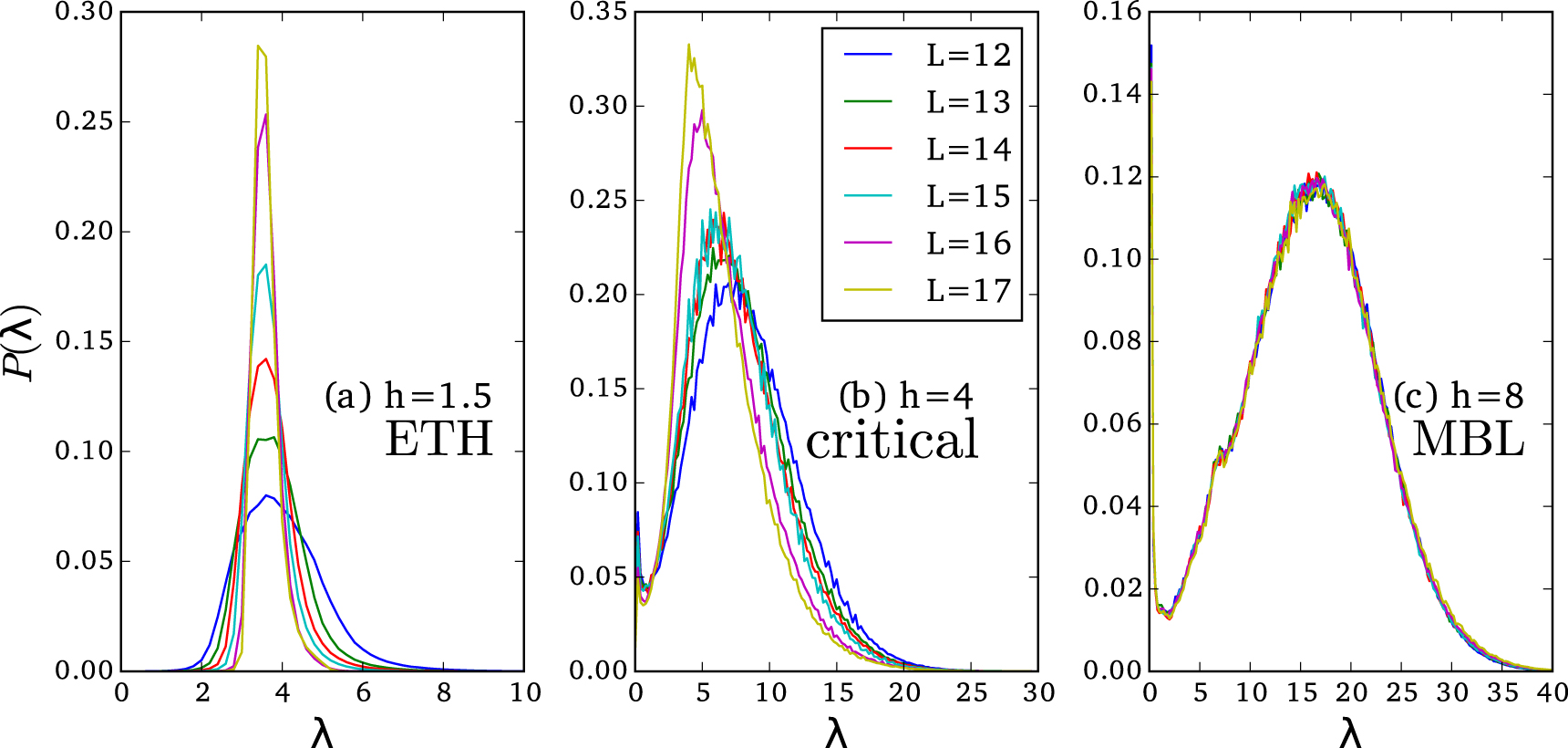
We begin by reviewing the relevant results of [43] on the properties of entanglement spectra in the ETH and MBL phases. The quantity we will be most interested in is the density of states (EDOS) of the entanglement spectrum, which was found to be qualitatively different in the two phases. Figure 2 shows examples of the EDOS in the ETH (a) and MBL (c) phases. To understand the ETH density of states, the prototypical example is a system at infinite temperature. In this case every eigenvalue of the reduced density matrix is equal. Let us define NA to be the size of the Hilbert space of the region A (the complement to which is traced out), and LA to be the length of this region in the one-dimensional systems we will study. Then  for all i. Since the systems we study are not at infinite temperature we instead get a density of states narrowly distributed around LA. In the MBL phase a model wavefunction could be a pure product state which has
  and all other
  . Away from this ideal limit we believe that the eigenstates should be products of 'l-bits', which decay exponentially in space. Therefore there will be some non-zero λ values which result from cutting the tails of these l-bits. From this intuition we expect an EDOS which decays exponentially from
  . However in [43] we showed that the majority of entanglement eigenvalues are not in this exponentially decaying part but are instead in another peak which is at much higher entanglement eigenvalue. The level spacings in this higher peak obey semi-Poisson statistics, which are indicative of criticality.

Figure 2. Entanglement density of states (EDOS) for phases in the thermal phase with  (a), in the critical phase with h = 4 (b), and in the MBL phase with h = 8 (c), for
  . In the thermal phase the EDOS is peaked around a value proportional to LA and independent of L. In the MBL phase the EDOS has two peaks, one which exponentially decays from zero and the other at higher entanglement energies. In the critical phase the system moves between the two cases as a function of L. The EDOs shown we obtained by averaging over the middle third of the eigenstates in 128−512 realizations of disorder.
Download figure:
Standard image High-resolution imageWe study the location of this 'high-energy peak', which turns out to be a very sensitive probe of the critical properties of the system. We have studied the scaling of the 'high energy peak' with system size L, subsystem size LA, and disorder strength h. We discuss these in turn. Note that we found that we need  in order to have good statistics. Since for any location of entanglement cut, LA is the smaller of the two subregions, it then follows that we need
  . Meanwhile, the largest system sizes we can access given available numerical resources are L = 17, and thus our results are limited to the range
  . A larger range may be accessible with specifically tailored models (e.g. [49]) or with greater computational resources, and would be an interesting problem for future work.
4. Results
4.1. System size dependence
Deep in either the thermal or MBL phases, we expect the EDOS to be independent of L. In the thermal phase, our intuition from the infinite-temperature case tells us that the EDOS should depend only on the number of degrees of freedom in the traced-out region A, i.e. it depends on LA but not on L. In the MBL phase the correlation length is very small. Increasing L for fixed LA means adding degrees of freedom far from the region A, and these should not affect the entanglement between A and the rest of the system. In figure 2 we show how the EDOS changes with system sizes for a few different disorder strengths. Deep in the thermal (a) and MBL phases (c) the EDOS peak position changes little with L, as expected. But at intermediate values of h (b), which we might expect to lie in the critical region, we see significant changes in the EDOS peak position as a function of L.
The dependence of the EDOS in the critical region has a natural explanation in terms of the scenario outlined in [37] (and anticipated also in [27]). In that work it was argued that entanglement in the critical regime is dominated by sparse 'fractal' networks of long range resonances. Adding degrees of freedom far away from the entanglement cut alters the structures of these resonant networks, and hence alters the EDOS. As we increase system size at subcritical disorder, tuning through the critical to thermal crossover, these 'resonant networks' densely fill in, so that EDOS becomes insensitive to system size as discussed above. Meanwhile, as we increase system size at supercritical disorder, tuning through the critical to MBL crossover, then eventually system size exceeds the size of the resonances, such that adding degrees of freedom far from the cut no longer affects the resonant networks across the entanglement cut, or the EDOS. The key diagnostic of criticality is thus a dependence of the EDOS on total system size L, at constant h and LA.
We can quantify the motion of the density of states with system size by tracking the position of the top of the high entanglement eigenvalue peak. In figure 3 we plot this peak location as a function of L for a variety of disorder strengths, at  . Note that the curves in this plot correspond to moving down vertical lines in figure 1. At small or large h the curves are flat, since at the system sizes we can access these disorder strengths are entirely in either the thermal or MBL phases. At intermediate disorder, e.g. h = 3, we see curves which decrease steadily, implying that at the system sizes we can access these curves are all in the critical regime. In figure 4 we show the results of fitting the data in figure 3 to straight lines, which shows a non-zero slope in the critical region which seems to decay to zero in both the small- and large-disorder limits.

Figure 3. The location of the maximum of the EDOS (excluding the peak around  which occurs in the MBL phase), as a function of L for several h values and
  . The peak location should only depend on L in the critical regime. Thus this plot allows us to identify both the critical-thermal boundary and the critical-MBL boundary. The peak location for a single sample was computed by averaging maximum values of the EDOS of all that sample's eigenstates (see section 4.4 for justification of this procedure). The plotted data and errors are the result of averaging the peak locations of 128−512 samples. (More samples were used at smaller sizes and larger disorder.) The separation between curves at different h is larger than the change in the curves with L, especially at large disorder. Therefore to show all data clearly on the same plot we subtracted a constant from each curve with
  . The following is a list of the values of to constants which were subtracted in the format (h:offset): (3.5:0.5), (4:1), (4.5:1.5), (5:2), (6:4), (7:5.5), (8:6.5), (9:7.5), (10:8.5), (12:10.5).
Download figure:
Standard image High-resolution image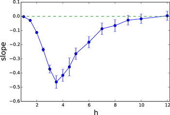
Figure 4. The slope of the best-fit lines to the data in figure 3. As expected, in the critical region the slope is large and negative while it tends to zero for both strong and weak disorder.
Download figure:
Standard image High-resolution imageThe data in figure 4 was the result of fitting all the data to a straight line, but if the picture in figure 1(a) is correct then the slope of such lines should decrease as L is increased (though it is possible that the range of L that we study is too narrow to observe this). If such a change occured we could imagine defining a 'crossover lengthscale'  for the quantum critical fan as the lengthscale where the dependence of the EDOS peak on L disappears. The observation of such a crossover at weak disorder sets a lower bound on the location of the thermal-MBL transition, while at strong disorder it would set an upper bound. The observation of such an upper bound in finite-size numerics would definitively rule out the scenario in figure 1(b).
We can clearly detect  at weak disorder, and we plot its observed values as green circles in figure 1, finding as expected that it moves to large L as h is increased. Interestingly, we also observe a flattening of the curves at
  , corresponding to
  , and we plot these results as green squares in figure 1.
We interpret this flattening as an observation of  ,
, 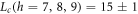 , and
, and  . This second crossover lengthscale, which is a decreasing function of disorder strength, corresponds to the right side of the quantum critical fan in figure 1, constituting to our knowledge the first observation of the critical to MBL crossover. We believe that the apparent 'uptick' in the peak position at large h and largest L is a numerical artifact (in this regime the curves are 'flat within error bars'), although it is interesting to speculate about a possible second crossover, which could modify the picture of the phase diagram in figure 1.
4.2. Dependence of entanglement spectra on subsystem size
We now explore how the peak position varies as a function of subsystem size LA, at fixed system size L. In the thermal phase the location of the peak in the EDOS should be  . In the MBL phase, we also expect the peak's location to scale as LA, by the following argument: most degrees of freedom live a distance
  away from the entanglement cut. (This is just dimensional analysis—LA is the only lengthscale characterizing the cut.) However, in the eigenstates degrees of freedom are typically only entangled within a lengthscale ξ, where ξ is the localization length. Given exponential localization, a degree of freedom a distance
  away from the cut will have entanglement
  across the cut, and thus will have entanglement eigenvalue
  . In figure 5 we show the peak location, as a function of LA for fixed L = 17 and several disorder strengths. We see that in the thermal phase the behavior is
  as expected (figure 5(a)). In the MBL phase the peak location scales approximately as LA, but there are small deviations from perfect linear behavior in the deep MBL regime (figure 5(b)). Understanding whether these deviations are physical, and to what physics they correspond if so, is an interesting challenge for future work.

Figure 5. The location of the maximum of the EDOS (excluding the peak around  which occurs in the MBL phase), as a function of LA for several h values and L = 16. As discussed in the text, the peak location grows
  in all phases. The data has been broken into multiple panels to make the small h behavior easy to see.
Download figure:
Standard image High-resolution image4.3. Dependence on disorder strength
We now consider the dependence on the disorder strength h. Note that our toy model above suggests that in the thermal phase, the peak location should be independent of h (depending only on LA), whereas in the MBL phase, peak location should be  . Now close to the transition,
  , whereas far from the transition (deep in the locator limit),
  . Given that exact diagonalization studies typically see
  [36], we should expect to see the peak location be (i) independent of h in the thermal regime (ii) increasing roughly linearly with h close to the MBL side of the transition, and (iii) increasing much more slowly with h in the deep MBL regime. In figure 6 we show the numerically obtained dependence of peak position on h for several system sizes. Note that the behavior is broadly consistent with the predictions of the toy model detailed above.

Figure 6. The location of the maximum of the EDOS (excluding the peak around  which occurs in the MBL phase), as a function of h for several L values and
  . In the ETH the curve is flat while the peak location is
  in the MBL phase.
Download figure:
Standard image High-resolution image4.4. Statistical fluctuations: variations between samples versus variations between eigenstates
In this subsection, we investigate the dominant source of the statistical fluctuations. In each sample we study, every eigenstate produces its own entanglement spectrum, and therefore its own entanglement density of states. Here we compare the density of states of eigenstates coming from the same sample to those from different samples. In addition to fundamental interest, it is important to understand these difference because they inform how we perform our data analysis.
Figure 7 shows such a comparison. To obtain this figure, we created a microcanonical average EDOS out of 1000 eigenstates of a single sample. At L = 14, where this data was taken, we focus  eigenstates (note that we restrict ourselves to the middle of the spectrum so that we do not have to worry about mobility edges), and therefore we can make five such different EDOS curves. We then repeat this procedure for multiple disorder realizations, with data coming from the same realization of disorder plotted in the same color. The plot shows that fluctuations between the EDOS obtained by microcanonical averaging over different energy windows within the same sample (different groups of 1000 eigenstates) are small compared to fluctuations between microcanonically averaged EDOS from different samples.

Figure 7. A comparison of EDOS for different groups of eigenstates in the same sample and in different samples. The curves in the figure are obtained by averaging over 1000 eigenstates, at h = 5,  , L = 14. Curves of the same color come from the same sample. We can see that distinct microcanonical averages of the EDOS from the same sample are much more similar than microcanonical averages from different samples, implying that sample-to-sample variation is more important than variation between microcanonical energy windows (of 1000 states) within the same sample.
Download figure:
Standard image High-resolution imageThese results inform our numerical procedures in a number of ways. For large system sizes we use the shift-invert method to obtain 1000 eigenstates in the middle of our spectrum, while for smaller system sizes we use full diagonalization. Figure 7 suggests that these methods should give very similar results, since the difference between EDOS obtianed from microcanonical averaging over different windows is much smaller than the fluctuations between samples. To confirm this expectation in figure 8 we show data for 256 samples, where each point is the result of averaging over 16 samples. The first four points (64 samples) were obtained using full diagonalization while the remainder we taken using shift-invert. If shift-invert gave different results we would expect larger error bars on the points taken with shift-invert, but we do not observe this.

Figure 8. Each data point in this figure is the result of averaging the peak locations of 8 different samples. For the first eight points (those on the left-hand side of the dashed line), all of the eigenstates of the samples were computed using full diagonalization, while in the remaining points only 1000 eigenstates in the middle of the spectrum were computed, using the shift-invert method. The different points are consistent (within error bars), and have error bars of similar size, which leads us to conclude that our results do not depend on whether we use shift-invert or full diagonalization. Data was taken for L = 14,  , h = 6.
Download figure:
Standard image High-resolution imagePreviously we computed the location of the EDOS peak by first computing an EDOS which is averaged over all eigenstates in a given sample, and then averaging those peak locations. We could imagine other ways of performing this analysis. We could compute the peak location for each eigenstate, and average those peak locations over eigenstates and samples. Figure 7 tells us that both of these averaging methods should give the same results, since the EDOS for all eigenstates in a given sample and the final error bar will be dominated by sample-to-sample fluctuations in any case. We could also imagine finding the peak of an EDOS which is averaged over all eigenstates and samples. The values of the peaks extracted this way will be different: in figure 7 for example one can see that the results of averaging the peaks of the different samples will not necessarily be the same as the peak of the average distribution. In figure 9 we show the results of extracting peak values from an EDOS averaged over all samples. To determine the values in figure 9 we fit the data near the top of the curve to a Gaussian distribution, and the peak location is the maximum of this fit. Using such a method it is less clear how to assign an error bar to our data, and furthermore the data seems more noisy than that in figure 3. However we can clearly see that this method gives similar results to those of figure 3.

Figure 9. Similar to figure 3, but using a different method of determining the average peak location (error bars not shown). Instead of finding a peak location for each sample and averaging those, we determine one EDOS by averaging over all samples and plot its peak value. Though the results of the two methods are qualitatively the same we find that the data using the full EDOS is noisier, and moreover it is harder to estimate error bars.
Download figure:
Standard image High-resolution image
5. Discussion
We have examined the MBL transition through the lens of the entanglement spectrum. In particular, we have shown that system size dependence of the high energy peak in the entanglement spectrum is a sensitive measure of criticality, which allows us to study both the critical to thermal crossover (which many studies have seen before), and the critical to MBL crossover (which has never before been observed to our knowledge). As such, not only does our work justify a picture in which at finite size the MBL and thermal regimes are separated by a 'critical' fan, but it also suggests both a lower and an upper bound on the critical disorder strength for the MBL transition. (Of course, while observation of a critical fan suggests a critical point between the bounds we place herein, it remains possible that e.g. rare region effects could render the critical point avoided in thermodynamically large samples.)
We provided two pieces of evidence suggesting that the entanglement spectrum can detect the critical-MBL crossover. The first was that at large disorder the peak location is independent of L, which is a qualitatively different behavior than the decrease of the peak location with L observed in the critical region. The second evidence was that for a given h we can observe a crossover lengthscale  where the peak location versus L curves become flat. If these results are correct this implies a critical-MBL crossover. However there is still work to be done to improve our results. Though figure 4 seems to show a curve which goes to zero at large h, we cannot rule out that it only asymptotically approaches zero. It may be desirable to apply greater computation resources (or new techniques) to this problem in an effort to more definitively establish whether the slope indeed vanishes. It is also possible that other systems, while exhibiting the same universal properties, might yield cleaner results at the system sizes we are able to study. We note that the data we present required thousands of hours of CPU time, so improving our data by obtaining more samples, though possible, would require significant computational resources. A similar problem exists with our putative observation of
  . It is possible that the flattening we observe is statistical noise, and higher-quality data could help us to establish this7
. Higher quality data might also provide a tighter bound on the location of the thermodynamic transition point (recall that our current data suggests
. It is possible that the flattening we observe is statistical noise, and higher-quality data could help us to establish this7
. Higher quality data might also provide a tighter bound on the location of the thermodynamic transition point (recall that our current data suggests  ). Also interesting would be to apply similar analyses for models with quasi-periodic disorder, which may also be relevant for understanding the MBL transition [50], or to examine the dynamical evolution of the entanglement spectrum starting from low entanglement initial conditions, as pioneered by [51].
Acknowledgments
We thank SA Parameswaran, R Vasseur, AC Potter, R N Bhatt and especially Vedika Khemani for feedback on the manuscript. RN is supported by the Foundational Questions Institute (fqxi.org; grant no. FQXi-RFP-1617) through their fund at the Silicon Valley Community Foundation. SDG is supported by Department of Energy BES Grant DE-SC0002140.
Footnotes
- 4
The transition also occurs as a function of energy density, in this work we will fix the energy density to be in the middle of the density of states.
- 5
And also LA.
- 6
What we have defined is the Von Neumann entanglement entropy, other entanglement entropies (e.g. Renyi) are defined similarly.
- 7
As a rought estimate, at e.g. h = 7 the probability to observe our data if the true results lie on a straight line (the p-value) is 0.08, which is suggestive but not definitive.