Subdiffraction incoherent optical imaging via spatial-mode demultiplexing

Recent research, initiated by our group [1–7], has shown that far-field linear optical methods can significantly improve the resolution of two equally bright incoherent optical point sources with sub-Rayleigh separations [1–15], overcoming previously established statistical limits [16–19]. The rapid experimental demonstrations [12–15] have heightened the promise of our approach. An open problem, of fundamental interest in optics and monumental importance to astronomy and fluorescence microscopy, is whether these results can be generalized for an arbitrary distribution of incoherent sources. Here I take a major step towards solving the problem by proposing a generalized spatial-mode demultiplexing (SPADE) measurement scheme and proving its superiority over direct imaging via a statistical analysis.

The use of coherent optical processing to improve the lateral resolution of incoherent imaging has thus far received only modest attention, as prior proposals [13, 20–25] either did not demonstrate any substantial improvement or neglected the important effect of noise. Using quantum optics and parameter estimation theory, here I show that, for any object too small to be resolved by diffraction-limited direct imaging, SPADE can estimate its second or higher moments much more precisely than direct imaging can fundamentally do in the presence of photon shot noise. Moreover, I prove that SPADE can approach the optimal precision allowed by quantum mechanics in estimating the location and scale parameters of a subdiffraction object. Given the usefulness of moments in identifying the size and shape of an object [26], the proposed scheme, realizable with far-field linear optics and photon counting, should provide a major boost to incoherent imaging applications that are limited by diffraction and photon shot noise, including not only fluorescence microscopy [27–30] and space-based telescopes [31] but also modern ground-based telescopes [32–35].

This paper is organized as follows. Section 2 introduces the background theory of quantum optics and parameter estimation for incoherent imaging. Section 3 describes the SPADE scheme for general imaging. Section 4 presents the most important results of this paper, namely, a comparison between the statistical performances of direct imaging and SPADE in the subdiffraction regime, showing the possibility of giant precision enhancements for moment estimation, while appendix justifies an approximation made in section 4 in more detail. Section 5 presents a numerical example to illustrate the theory, comparing the errors in estimating the first and second moments of subdiffraction objects using direct imaging and SPADE. Section 6 proves that SPADE is close to the quantum precision limits to location and scale estimation in the subdiffraction regime. Section 7 discusses other practical and open issues.

2.1. Quantum optics

I begin with the quantum formalism established in [1] to ensure correct physics. The quantum state of thermal light with M temporal modes and a bandwidth much smaller than the center frequency can be written as ${\rho }^{\otimes M}$, where

$$\begin{eqnarray}&&\rho =(1-\epsilon ){\rho }_{0}+\epsilon {\rho }_{1}+O({\epsilon }^{2}),\end{eqnarray} \tag{ 2.1 }$$

$\epsilon$ is the average photon number per mode assumed to be $\ll 1$ [36, 37], ${\rho }_{0}=| {\rm{vac}}\rangle \langle {\rm{vac}}|$ is the vacuum state, ${\rho }_{1}$ is the one-photon state with a density matrix equal to the mutual coherence function, and $O({\epsilon }^{2})$ denotes second-order terms, which are neglected hereafter. It is standard to assume that the fields from incoherent objects, such as stellar or fluorescent emitters, are spatially uncorrelated at the source [37]. In a diffraction-limited imaging system, the fields then propagate as waves; the Van Cittert-Zernike theorem is the most venerable consequence [37]. At the image plane of a conventional lens-based two-dimensional imaging system in the paraxial regime [37, 38], this implies

$$\begin{eqnarray}&&{\rho }_{1}=\int {{\rm{d}}}^{2}{\boldsymbol{R}}F({\boldsymbol{R}})| {\psi }_{{\boldsymbol{R}}}\rangle \langle {\psi }_{{\boldsymbol{R}}}| ,\qquad \qquad | {\psi }_{{\boldsymbol{R}}}\rangle =\int {{\rm{d}}}^{2}{\boldsymbol{r}}\psi ({\boldsymbol{r}}-{\boldsymbol{R}})| {\boldsymbol{r}}\rangle ,\end{eqnarray} \tag{ 2.2 }$$

where ${\boldsymbol{R}}=(X,Y)$ is the object-plane position, the notation $({u}_{1},{u}_{2},\ldots )$ denotes a column vector, $F({\boldsymbol{R}})$ is the source intensity distribution with normalization $\int {{\rm{d}}}^{2}{\boldsymbol{R}}F({\boldsymbol{R}})=1$, $| {\boldsymbol{r}}\rangle ={a}^{\dagger }({\boldsymbol{r}})| {\rm{vac}}\rangle$ is a one-photon position eigenket on the image plane at position ${\boldsymbol{r}}=(x,y)$ with $[a({\boldsymbol{r}}),{a}^{\dagger }({\boldsymbol{r}}^{\prime} )]={\delta }^{2}({\boldsymbol{r}}-{\boldsymbol{r}}^{\prime} )$ [39], and $\psi ({\boldsymbol{r}})$ is the field point-spread function (PSF) of the imaging system. Without loss of generality, the image-plane position vector ${\boldsymbol{r}}$ has been scaled with respect to the magnification to follow the same scale as ${\boldsymbol{R}}$ [38]. For convenience, I also normalize the position vectors with respect to the width of the PSF to make them dimensionless.

Consider the processing and measurement of the image-plane field by linear optics and photon counting. The counting distribution for each ρ can be expressed as $\langle {n}_{0},{n}_{1},\ldots | \rho | {n}_{0},{n}_{1},\ldots \rangle$, where $| {n}_{0},{n}_{1},\ldots \rangle =({\prod }_{j=0}^{\infty }{b}_{j}^{\dagger {n}_{j}}/\sqrt{{n}_{j}!})| {\rm{vac}}\rangle$, ${b}_{j}\equiv \int {{\rm{d}}}^{2}{\boldsymbol{r}}{\phi }_{j}^{* }({\boldsymbol{r}})a({\boldsymbol{r}})$, ${\phi }_{j}({\boldsymbol{r}})$ is the optical mode function that is projected to the jth output, and $[{b}_{j},{b}_{k}^{\dagger }]=\int {{\rm{d}}}^{2}{\boldsymbol{r}}{\phi }_{j}^{* }({\boldsymbol{r}}){\phi }_{k}({\boldsymbol{r}})={\delta }_{{jk}}$. With the negligence of multiphoton coincidences, the relevant projections are $\{| {\rm{vac}}\rangle ,| {\phi }_{j}\rangle \}$, with $| {\phi }_{j}\rangle \equiv | 0,\ldots ,{n}_{j}=1,\ldots ,0\rangle ={b}_{j}^{\dagger }| {\rm{vac}}\rangle =\int {{\rm{d}}}^{2}{\boldsymbol{r}}{\phi }_{j}({\boldsymbol{r}})| {\boldsymbol{r}}\rangle$. The zero-photon probability becomes $1-\epsilon$ and the probability of one photon being detected in the jth mode becomes $\epsilon p(j)$, where

$$\begin{eqnarray}&&p(j)\equiv \langle {\phi }_{j}| {\rho }_{1}| {\phi }_{j}\rangle =\int {{\rm{d}}}^{2}{\boldsymbol{R}}F({\boldsymbol{R}}){| \langle {\phi }_{j}| {\psi }_{{\boldsymbol{R}}}\rangle | }^{2}\end{eqnarray} \tag{ 2.3 }$$

is the one-photon distribution. A generalization of the measurement model using the concept of positive operator-valued measures is possible [1, 3] but not needed here.

For example, direct imaging can be idealized as a measurement of the position of each photon, leading to an expected image given by

$$\begin{eqnarray}&&f({\boldsymbol{r}})\equiv \langle {\boldsymbol{r}}| {\rho }_{1}| {\boldsymbol{r}}\rangle =\int {{\rm{d}}}^{2}{\boldsymbol{R}}F({\boldsymbol{R}}){| \psi ({\boldsymbol{r}}-{\boldsymbol{R}})| }^{2},\end{eqnarray} \tag{ 2.4 }$$

which is a basic result in statistical optics [37, 38]. While equation (2.4) suggests that, similar to the coherent-imaging formalism, the PSF acts as a low-pass filter in the spatial frequency domain [38], the effect of more general optical processing according to equation (2.3) is more subtle and offers surprising advantages, as demonstrated by recent work [1–15] and elaborated in this paper.

Over M temporal modes, the probability distribution of photon numbers $m=({m}_{0},{m}_{1},\ldots )$ detected in the respective optical modes becomes

$$\begin{eqnarray}&&P(m)=\displaystyle \sum _{L}{ \mathcal M }(m| L){ \mathcal B }(L),\end{eqnarray} \tag{ 2.5 }$$

where ${ \mathcal B }(L)$ is the binomial distribution for detecting L photons over M trials with single-trial success probability $\epsilon$ and ${ \mathcal M }(m| L)={\delta }_{L,{\sum }_{j}{m}_{j}}L!{\prod }_{j}{[p(j)]}^{{m}_{j}}/{m}_{j}!$ is the multinomial distribution of m given L total photons [40]. The average photon number in all modes becomes $N\equiv M\epsilon .$ Taking the limit of $\epsilon \to 0$ while holding N constant, ${ \mathcal B }(L)$ becomes Poisson with mean N, and $P(m)\to \exp (-N){\prod }_{j}{[{Np}(j)]}^{{m}_{j}}/{m}_{j}!$, which is the widely used Poisson model of photon counting for incoherent sources at optical frequencies [3, 18, 27–31, 36].

2.2. Parameter estimation

The central goal of imaging is to infer unknown properties of the source distribution $F({\boldsymbol{R}})$ from the measurement outcome m. Here I frame it as a parameter estimation problem, defining $\theta =({\theta }_{1},{\theta }_{2},\ldots )$ as a column vector of unknown parameters and assuming the source distribution $F({\boldsymbol{R}}| \theta )$ to be a function of θ. Denote an estimator as $\check{\theta }(m)$ and its error covariance matrix as ${{\rm{\Sigma }}}_{\mu \nu }(\theta )={\sum }_{m}P(m| \theta )[{\check{\theta }}_{\mu }(m)-{\theta }_{\mu }][{\check{\theta }}_{\nu }(m)-{\theta }_{\nu }]$. For any unbiased estimator (${\sum }_{m}\check{\theta }(m)P(m| \theta )=\theta$), the Cramér-Rao bound (CRB) is given by [40, 41]

$$\begin{eqnarray}&&{\rm{\Sigma }}(\theta )\geqslant {\rm{CRB}}(\theta )\equiv {J}^{-1}(\theta ),\end{eqnarray} \tag{ 2.6 }$$

where $J(\theta )$ is the Fisher information matrix and the matrix inequality implies that ${\rm{\Sigma }}-{J}^{-1}$ is positive-semidefinite, or equivalently ${u}^{\top }({\rm{\Sigma }}-{J}^{-1})u\geqslant 0$ for any real vector u. Assuming the model given by equation (2.5) and a known N, it can be shown [3] that

$$\begin{eqnarray}&&{J}_{\mu \nu }(\theta )=N\displaystyle \sum _{j}\displaystyle \frac{1}{p(j| \theta )}\displaystyle \frac{\partial p(j| \theta )}{\partial {\theta }_{\mu }}\displaystyle \frac{\partial p(j| \theta )}{\partial {\theta }_{\nu }},\end{eqnarray} \tag{ 2.7 }$$

which is a well known expression [16–18, 28, 30, 36]. For example, the direct-imaging information, given equation (2.4) and the limit $p(j| \theta )\to {d}^{2}{\boldsymbol{r}}f({\boldsymbol{r}}| \theta )$, is

$$\begin{eqnarray}&&{J}_{\mu \nu }^{({\rm{direct}})}(\theta )=N\int {{\rm{d}}}^{2}{\boldsymbol{r}}\displaystyle \frac{1}{f({\boldsymbol{r}}| \theta )}\displaystyle \frac{\partial f({\boldsymbol{r}}| \theta )}{\partial {\theta }_{\mu }}\displaystyle \frac{\partial f({\boldsymbol{r}}| \theta )}{\partial {\theta }_{\nu }}.\end{eqnarray} \tag{ 2.8 }$$

For large N, the maximum-likelihood estimator is asymptotically normal with mean θ and covariance ${\rm{\Sigma }}(\theta )={J}^{-1}(\theta )$, even though it may be biased for finite N [40, 41]. Bayesian and minimax generalizations of the CRB for any biased or unbiased estimator are possible [5, 41] but not considered here as they offer qualitatively similar conclusions. The Fisher information is nowadays regarded as the standard precision measure in incoherent imaging research, especially in fluorescence microscopy [18, 28–30], where photon shot noise is the dominant noise source and a proper statistical analysis is essential.

Apart from the CRB, another useful property of the Fisher information is the data-processing inequality [42, 43], which mandates that, once the measurement is made, no further processing of the data can increase the information. For example, direct imaging with large pixels can be modeled as integrations of photon counts over groups of infinitesimally small pixels, so the information can never exceed equation (2.8). More generally, the data-processing inequality rules out the possibility of improving the information using any processing that applies to the direct-imaging intensity, such as the proposal by Walker et al for incoherent imaging in [20], even if the processing is done with optics. Hence, as argued by Tham et al [14], coherent processing that is sensitive to the phase of the field is the only way to improve upon equation (2.8). The information for any coherent processing and measurement is in turn limited by quantum upper bounds in terms of ${\rho }_{1}$ [1, 3, 6, 43–46].

SPADE is a technique previously proposed for the purpose of superresolving the separation between two incoherent point sources [1, 6, 7, 9, 13–15]. I now ask how SPADE can be generalized for the imaging of an arbitrary source distribution. Consider the transverse-electromagnetic (TEM) basis $\{| {\boldsymbol{q}}\rangle ;{\boldsymbol{q}}=({q}_{x},{q}_{y})\in {{\mathbb{N}}}^{2}\}$ [47], where

$$\begin{eqnarray}&&| {\boldsymbol{q}}\rangle =\int {{\rm{d}}}^{2}{\boldsymbol{r}}{\phi }_{{\boldsymbol{q}}}({\boldsymbol{r}})| {\boldsymbol{r}}\rangle ,\end{eqnarray} \tag{ 3.1 }$$

$$\begin{eqnarray}&&{\phi }_{{\boldsymbol{q}}}({\boldsymbol{r}})\equiv \displaystyle \frac{{\mathrm{He}}_{{q}_{x}}(x){\mathrm{He}}_{{q}_{y}}(y)}{\sqrt{2\pi {q}_{x}!{q}_{y}!}}\exp \left(-\displaystyle \frac{{x}^{2}+{y}^{2}}{4}\right),\end{eqnarray} \tag{ 3.2 }$$

and ${\mathrm{He}}_{q}$ is the Hermite polynomial [48, 49]. Assuming a Gaussian PSF given by $\psi ({\boldsymbol{r}})={\phi }_{00}({\boldsymbol{r}})$, which is a common assumption in fluorescence microscopy [28, 30], $| {\psi }_{{\boldsymbol{R}}}\rangle$ is a coherent state [50], and the one-photon density matrix in the TEM basis becomes

$$\begin{eqnarray}&&g({\boldsymbol{q}},{\boldsymbol{q}}^{\prime} | \theta )\equiv \langle {\boldsymbol{q}}| {\rho }_{1}(\theta )| {\boldsymbol{q}}^{\prime} \rangle \end{eqnarray} \tag{ 3.3 }$$

$$\begin{eqnarray}&&=\,C({\boldsymbol{q}},{\boldsymbol{q}}^{\prime} )\int {{\rm{d}}}^{2}{\boldsymbol{R}}F({\boldsymbol{R}}| \theta ){e}^{-({X}^{2}+{Y}^{2})/4}{X}^{{q}_{x}+{q}_{x}^{\prime }}{Y}^{{q}_{y}+{q}_{y}^{\prime }},\end{eqnarray} \tag{ 3.4 }$$

where

$$\begin{eqnarray}&&C({\boldsymbol{q}},{\boldsymbol{q}}^{\prime} )\equiv \displaystyle \frac{1}{{2}^{| {\boldsymbol{q}}+{\boldsymbol{q}}^{\prime} {| }_{1}}\sqrt{{\boldsymbol{q}}!{\boldsymbol{q}}^{\prime} !}},\qquad | {\boldsymbol{q}}{| }_{1}\equiv {q}_{x}+{q}_{y},\qquad {\boldsymbol{q}}!\equiv {q}_{x}!{q}_{y}!.\end{eqnarray} \tag{ 3.5 }$$

To investigate the imaging capability of SPADE measurements, define

$$\begin{eqnarray}&&{{\rm{\Theta }}}_{{\boldsymbol{\mu }}}(\theta )\equiv \int {{\rm{d}}}^{2}{\boldsymbol{R}}F({\boldsymbol{R}}| \theta ){e}^{-({X}^{2}+{Y}^{2})/4}{X}^{{\mu }_{X}}{Y}^{{\mu }_{Y}},\end{eqnarray} \tag{ 3.6 }$$

with ${\boldsymbol{\mu }}=({\mu }_{X},{\mu }_{Y})$, leading to a linear parameterization of g given by

$$\begin{eqnarray}&&g({\boldsymbol{q}},{\boldsymbol{q}}^{\prime} | \theta )=C({\boldsymbol{q}},{\boldsymbol{q}}^{\prime} ){{\rm{\Theta }}}_{{\boldsymbol{q}}+{\boldsymbol{q}}^{\prime} }.\end{eqnarray} \tag{ 3.7 }$$

Notice that each ${{\rm{\Theta }}}_{{\boldsymbol{\mu }}}$ is a moment of the source distribution filtered by a Gaussian. In particular, if the object is much smaller than the PSF width, the Gaussian can be neglected, and ${{\rm{\Theta }}}_{{\boldsymbol{\mu }}}$ becomes a moment of the source distribution itself. This subdiffraction regime is of central interest to superresolution imaging and, as shown in section 4, also a regime in which direct imaging performs relatively poorly. Since a distribution is uniquely determined by its moments [51], $F({\boldsymbol{R}}| \theta )\exp [-({X}^{2}+{Y}^{2})/4]$ and therefore $F({\boldsymbol{R}}| \theta )$ can be reconstructed given the moments, at least in principle. Note also that the object-moment order ${\boldsymbol{\mu }}$ is nontrivially related to the order of the matrix element via ${\boldsymbol{\mu }}={\boldsymbol{q}}+{\boldsymbol{q}}^{\prime}$, which is a peculiar feature of incoherent imaging.

A measurement in the TEM basis yields

$$\begin{eqnarray}&&{p}^{({\rm{TEM}})}({\boldsymbol{q}}| \theta )=C({\boldsymbol{q}},{\boldsymbol{q}}){{\rm{\Theta }}}_{2{\boldsymbol{q}}},\end{eqnarray} \tag{ 3.8 }$$

which is sensitive only to moments with even ${\mu }_{X}$ and ${\mu }_{Y}$, as also recognized by Yang et al in [13]. This measurement is realized by demultiplexing the image-plane optical field in terms of the TEM basis via linear optics before photon counting for each mode and can be implemented by many methods, most commonly found in optical communications [1, 6, 15, 52–54]. To access the other moments, consider interferometry between two TEM modes that implements the projections

$$\begin{eqnarray}&&| +\rangle \equiv \displaystyle \frac{1}{\sqrt{2}}(| {\boldsymbol{q}}\rangle +| {\boldsymbol{q}}^{\prime} \rangle ),\qquad \qquad | -\rangle \equiv \displaystyle \frac{1}{\sqrt{2}}(| {\boldsymbol{q}}\rangle -| {\boldsymbol{q}}^{\prime} \rangle ).\end{eqnarray} \tag{ 3.9 }$$

This two-channel interferometric TEM (iTEM) measurement leads to

$$\begin{eqnarray}{p}^{({\boldsymbol{q}},{\boldsymbol{q}}^{\prime} )}(+| \theta ) & = & \beta ({\boldsymbol{q}},{\boldsymbol{q}}^{\prime} )+C({\boldsymbol{q}},{\boldsymbol{q}}^{\prime} ){{\rm{\Theta }}}_{{\boldsymbol{q}}+{\boldsymbol{q}}^{\prime} },\\ {p}^{({\boldsymbol{q}},{\boldsymbol{q}}^{\prime} )}(-| \theta ) & = & \beta ({\boldsymbol{q}},{\boldsymbol{q}}^{\prime} )-C({\boldsymbol{q}},{\boldsymbol{q}}^{\prime} ){{\rm{\Theta }}}_{{\boldsymbol{q}}+{\boldsymbol{q}}^{\prime} },\end{eqnarray} \tag{ 3.10 }$$

$$\begin{eqnarray}&&\beta ({\boldsymbol{q}},{\boldsymbol{q}}^{\prime} )\equiv \displaystyle \frac{1}{2}[C({\boldsymbol{q}},{\boldsymbol{q}}){{\rm{\Theta }}}_{2{\boldsymbol{q}}}+C({\boldsymbol{q}}^{\prime} ,{\boldsymbol{q}}^{\prime} ){{\rm{\Theta }}}_{2{\boldsymbol{q}}^{\prime} }].\end{eqnarray} \tag{ 3.11 }$$

The dependence on ${{\rm{\Theta }}}_{{\boldsymbol{q}}+{\boldsymbol{q}}^{\prime} }$ is the main interest here, as it allows one to access any moment parameter.

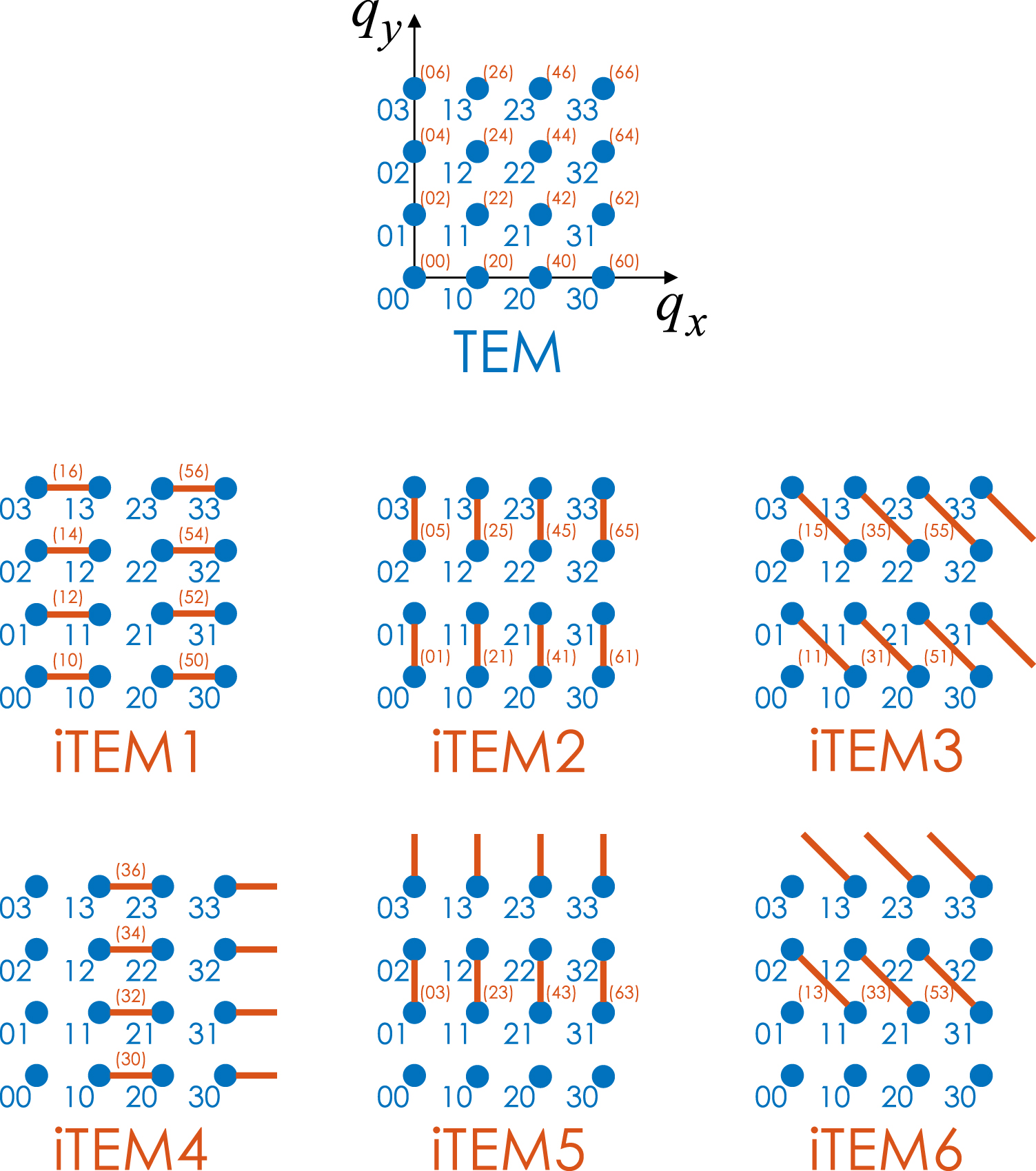
For multiparameter estimation and general imaging, multiple TEM and iTEM measurements are needed. To be specific, table 1 lists a set of schemes that can be used together to estimate all the moment parameters, while figure 1 shows a graphical representation of the schemes in the $({q}_{x},{q}_{y})$ space. Neighboring modes are used in the proposed iTEM schemes because they maximize the Fisher information, as shown later in section 4. The bases in different schemes are incompatible with one another, so the photons have to be rationed among the 7 schemes, by applying the different schemes sequentially through reprogrammable interferometers or spatial-light modulators [15, 52–54] for example.

Zoom In Zoom Out Reset image size

Table 1.  A list of measurement schemes, their projections, and the orders ${\boldsymbol{\mu }}=({\mu }_{X},{\mu }_{Y})$ of the moment parameters ${{\rm{\Theta }}}_{{\boldsymbol{\mu }}}$ to which they are sensitive.

Scheme	Projections	qx	qy	${\mu }_{X}$	${\mu }_{Y}$
TEM	$| {\boldsymbol{q}}\rangle$	${\mathbb{N}}$	${\mathbb{N}}$	even	even
iTEM1	$[| {\boldsymbol{q}}\rangle \pm | {\boldsymbol{q}}+(1,0)\rangle ]/\sqrt{2}$	even	${\mathbb{N}}$	$1,5,\ldots$	even
iTEM2	$[| {\boldsymbol{q}}\rangle \pm | {\boldsymbol{q}}+(0,1)\rangle ]/\sqrt{2}$	${\mathbb{N}}$	even	even	$1,5,\ldots$
iTEM3	$[| {\boldsymbol{q}}\rangle \pm | {\boldsymbol{q}}+(1,-1)\rangle ]/\sqrt{2}$	${\mathbb{N}}$	odd	odd	$1,5,\ldots$
iTEM4	$[| {\boldsymbol{q}}\rangle \pm | {\boldsymbol{q}}+(1,0)\rangle ]/\sqrt{2}$	odd	${\mathbb{N}}$	$3,7,\ldots$	even
iTEM5	$[| {\boldsymbol{q}}\rangle \pm | {\boldsymbol{q}}+(0,1)\rangle ]/\sqrt{2}$	${\mathbb{N}}$	odd	even	$3,7,\ldots$
iTEM6	$[| {\boldsymbol{q}}\rangle \pm | {\boldsymbol{q}}+(1,-1)\rangle ]/\sqrt{2}$	${\mathbb{N}}$	even	odd	$3,7,\ldots$

4.1. Direct imaging

Although the proposed SPADE method can in principle perform general imaging, its complexity would not be justifiable if it could not offer any significant advantage over direct imaging. To compare their statistical performances, consider first direct imaging with a Gaussian PSF. Expanding $| \psi ({\boldsymbol{r}}-{\boldsymbol{R}}){| }^{2}$ in a Taylor series, I obtain

$$\begin{eqnarray}&&f({\boldsymbol{r}}| \theta )={| {\phi }_{00}({\boldsymbol{r}})| }^{2}\left[1+\displaystyle \sum _{{\boldsymbol{\mu }}}{D}_{{\boldsymbol{\mu }}}({\boldsymbol{r}}){\theta }_{{\boldsymbol{\mu }}}\right],\end{eqnarray} \tag{ 4.1 }$$

$$\begin{eqnarray}&&{D}_{{\boldsymbol{\mu }}}({\boldsymbol{r}})\equiv \displaystyle \frac{{\mathrm{He}}_{{\mu }_{X}}(x){\mathrm{He}}_{{\mu }_{Y}}(y)}{{\boldsymbol{\mu }}!},\end{eqnarray} \tag{ 4.2 }$$

in terms of the moment parameters defined as

$$\begin{eqnarray}&&{\theta }_{{\boldsymbol{\mu }}}\equiv \int {{\rm{d}}}^{2}{\boldsymbol{R}}F({\boldsymbol{R}}| \theta ){X}^{{\mu }_{X}}{Y}^{{\mu }_{Y}}.\end{eqnarray} \tag{ 4.3 }$$

In terms of this parameterization, the Fisher information becomes

$$\begin{eqnarray}&&{J}_{{\boldsymbol{\mu }}{\boldsymbol{\nu }}}^{({\rm{direct}})}=N\int {{\rm{d}}}^{2}{\boldsymbol{r}}{| {\phi }_{00}({\boldsymbol{r}})| }^{2}\displaystyle \frac{{D}_{{\boldsymbol{\mu }}}({\boldsymbol{r}}){D}_{{\boldsymbol{\nu }}}({\boldsymbol{r}})}{1+{\displaystyle \sum }_{{\boldsymbol{\eta }}}{D}_{{\boldsymbol{\eta }}}({\boldsymbol{r}}){\theta }_{{\boldsymbol{\eta }}}}.\end{eqnarray} \tag{ 4.4 }$$

Assume now that the support of the source distribution is centered at the origin and has a maximum width Δ much smaller than the PSF width. Since the spatial dimensions have been normalized with respect to the PSF width, the PSF width is 1 in the dimensionless unit, and the assumption can be expressed as

$$\begin{eqnarray}&&{\rm{\Delta }}\ll 1,\end{eqnarray} \tag{ 4.5 }$$

which defines the subdiffraction regime. The parameters are then bounded by

$$\begin{eqnarray}&&| {\theta }_{{\boldsymbol{\mu }}}| \leqslant {\left(\displaystyle \frac{{\rm{\Delta }}}{2}\right)}^{| {\boldsymbol{\mu }}{| }_{1}},\end{eqnarray} \tag{ 4.6 }$$

and the image is so blurred that it resembles the TEM₀₀ mode rather than the object, viz., $f({\boldsymbol{r}}| \theta )={| {\phi }_{00}({\boldsymbol{r}})| }^{2}[1+O({\rm{\Delta }})]$. Writing the denominator in equation (4.4) as $1+O({\rm{\Delta }})$ and applying the orthogonality of Hermite polynomials [48, 49], I obtain

$$\begin{eqnarray}&&{J}_{{\boldsymbol{\mu }}{\boldsymbol{\nu }}}^{({\rm{direct}})}=\displaystyle \frac{N}{{\boldsymbol{\mu }}!}[{\delta }_{{\boldsymbol{\mu }}{\boldsymbol{\nu }}}+O({\rm{\Delta }})],\end{eqnarray} \tag{ 4.7 }$$

$$\begin{eqnarray}&&{{\rm{CRB}}}_{{\boldsymbol{\mu }}{\boldsymbol{\mu }}}^{({\rm{direct}})}=\displaystyle \frac{{\boldsymbol{\mu }}!}{N}[1+O({\rm{\Delta }})].\end{eqnarray} \tag{ 4.8 }$$

This is a significant result in its own right, as it establishes a fundamental limit to superresolution algorithms for shot-noise-limited direct imaging [20, 55–57], generalizing the earlier results for two sources [16–18] and establishing that, at least for a Gaussian PSF, the moments are a natural, approximately orthogonal [58] set of parameters for subdiffraction objects.

4.2. SPADE

To investigate the performance of SPADE for moment estimation, note that, in the subdiffraction regime, equation (3.6) can be expressed as

$$\begin{eqnarray}&&{{\rm{\Theta }}}_{{\boldsymbol{\mu }}}={\theta }_{{\boldsymbol{\mu }}}+O({{\rm{\Delta }}}^{| {\boldsymbol{\mu }}{| }_{1}+2}),\end{eqnarray} \tag{ 4.9 }$$

where $O({{\rm{\Delta }}}^{| {\boldsymbol{\mu }}{| }_{1}+2})$ is a linear combination of moments that are at least two orders above ${\boldsymbol{\mu }}$ and therefore much smaller than ${\theta }_{{\boldsymbol{\mu }}}$. Approximating ${{\rm{\Theta }}}_{{\boldsymbol{\mu }}}$ with ${\theta }_{{\boldsymbol{\mu }}}$ greatly simplifies the analysis below; appendix contains a more detailed justification of this approximation. For the TEM scheme, taking ${{\rm{\Theta }}}_{2{\boldsymbol{q}}}={\theta }_{2{\boldsymbol{q}}}$ in equation (3.8) makes the information matrix diagonal, with the nonzero elements given by

$$\begin{eqnarray}&&{J}_{{\boldsymbol{\mu }}{\boldsymbol{\mu }}}^{({\rm{TEM}})}=\displaystyle \frac{{N}^{({\rm{TEM}})}C({\boldsymbol{q}},{\boldsymbol{q}})}{{\theta }_{2{\boldsymbol{q}}}},\quad {\boldsymbol{\mu }}=2{\boldsymbol{q}},\end{eqnarray} \tag{ 4.10 }$$

where ${N}^{({\rm{TEM}})}$ is the average photon number available to the TEM scheme. The relevant CRB components are hence

$$\begin{eqnarray}&&{{\rm{CRB}}}_{{\boldsymbol{\mu }}{\boldsymbol{\mu }}}^{({\rm{TEM}})}=\displaystyle \frac{{\theta }_{2{\boldsymbol{q}}}}{{N}^{({\rm{TEM}})}C({\boldsymbol{q}},{\boldsymbol{q}})},\quad {\boldsymbol{\mu }}=2{\boldsymbol{q}}.\end{eqnarray} \tag{ 4.11 }$$

Defining the photon count of the ${\boldsymbol{q}}$th channel as ${m}_{{\boldsymbol{q}}}$ with expected value ${N}^{({\rm{TEM}})}{p}^{({\rm{TEM}})}({\boldsymbol{q}}| \theta )$, it is straightforward to show that the estimator

$$\begin{eqnarray}&&{\check{\theta }}_{2{\boldsymbol{q}}}=\displaystyle \frac{{m}_{{\boldsymbol{q}}}}{{N}^{({\rm{TEM}})}C({\boldsymbol{q}},{\boldsymbol{q}})}\end{eqnarray} \tag{ 4.12 }$$

is unbiased and achieves the error given by equation (4.11) under the assumption ${{\rm{\Theta }}}_{2{\boldsymbol{q}}}={\theta }_{2{\boldsymbol{q}}}$.

A precision enhancement factor can be defined as the ratio of equations (4.8) to (4.11), viz.,

$$\begin{eqnarray}&&\displaystyle \frac{{{\rm{CRB}}}_{{\boldsymbol{\mu }}{\boldsymbol{\mu }}}^{({\rm{direct}})}}{{{\rm{CRB}}}_{{\boldsymbol{\mu }}{\boldsymbol{\mu }}}^{({\rm{TEM}})}}\approx \displaystyle \frac{{N}^{({\rm{TEM}})}}{N}\displaystyle \frac{{\boldsymbol{\mu }}!}{{2}^{| {\boldsymbol{\mu }}{| }_{1}}({\boldsymbol{\mu }}/2)!{\theta }_{{\boldsymbol{\mu }}}}.\end{eqnarray} \tag{ 4.13 }$$

Apart from a factor ${N}^{({\rm{TEM}})}/N$ determined by the different photon numbers detectable in each method, the important point is that the factor scales inversely with ${\theta }_{{\boldsymbol{\mu }}}=O({{\rm{\Delta }}}^{| {\boldsymbol{\mu }}{| }_{1}})$, so the enhancement is enormous in the ${\rm{\Delta }}\ll 1$ subdiffraction regime. The prefactor in equation (4.13) also increases with increasing ${\boldsymbol{\mu }}$.

To investigate the errors in estimating the other moments via the iTEM schemes, assume ${{\rm{\Theta }}}_{{\boldsymbol{q}}+{\boldsymbol{q}}^{\prime} }={\theta }_{{\boldsymbol{q}}+{\boldsymbol{q}}^{\prime} }$ in equations (3.10). The dependence of equations (3.10) on ${\theta }_{{\boldsymbol{q}}+{\boldsymbol{q}}^{\prime} }$ is the main interest, while I treat $\beta ({\boldsymbol{q}},{\boldsymbol{q}}^{\prime} )$ as an unknown nuisance parameter [59]; the TEM scheme can offer additional information about $\beta ({\boldsymbol{q}},{\boldsymbol{q}}^{\prime} )$ via ${\theta }_{2{\boldsymbol{q}}}$ and ${\theta }_{2{\boldsymbol{q}}^{\prime} }$ but it is insignificant and neglected here to simplify the analysis. The information matrix with respect to $\{{\theta }_{{\boldsymbol{q}}+{\boldsymbol{q}}^{\prime} },\beta ({\boldsymbol{q}},{\boldsymbol{q}}^{\prime} )\}$ is block-diagonal and consists of a series of two-by-two matrices, each of which can be determined from equations (3.10) for two parameters $({\theta }_{{\boldsymbol{q}}+{\boldsymbol{q}}^{\prime} },\beta ({\boldsymbol{q}},{\boldsymbol{q}}^{\prime} ))$ and is given by

$$\begin{eqnarray}{J}^{({\boldsymbol{q}},{\boldsymbol{q}}^{\prime} )}=\displaystyle \frac{2{N}^{({\rm{iTEM}})}}{{\beta }^{2}({\boldsymbol{q}},{\boldsymbol{q}}^{\prime} )-{C}^{2}({\boldsymbol{q}},{\boldsymbol{q}}^{\prime} ){\theta }_{{\boldsymbol{q}}+{\boldsymbol{q}}^{\prime} }^{2}}\left(\begin{array}{cc}\beta ({\boldsymbol{q}},{\boldsymbol{q}}^{\prime} ){C}^{2}({\boldsymbol{q}},{\boldsymbol{q}}^{\prime} ) & -{C}^{2}({\boldsymbol{q}},{\boldsymbol{q}}^{\prime} ){\theta }_{{\boldsymbol{q}}+{\boldsymbol{q}}^{\prime} }\\ -{C}^{2}({\boldsymbol{q}},{\boldsymbol{q}}^{\prime} ){\theta }_{{\boldsymbol{q}}+{\boldsymbol{q}}^{\prime} } & \beta ({\boldsymbol{q}},{\boldsymbol{q}}^{\prime} )\end{array}\right),\end{eqnarray} \tag{ 4.14 }$$

where ${N}^{({\rm{iTEM}})}$ is the average photon number available to the iTEM scheme. The CRB component with respect to ${\theta }_{{\boldsymbol{q}}+{\boldsymbol{q}}^{\prime} }$ is hence obtained by taking the inverse of equation (4.14) and extracting the relevant term; the result is

$$\begin{eqnarray}&&{{\rm{CRB}}}_{{\boldsymbol{\mu }}{\boldsymbol{\mu }}}^{({\rm{iTEM}})}=\displaystyle \frac{\beta ({\boldsymbol{q}},{\boldsymbol{q}}^{\prime} )}{2{N}^{({\rm{iTEM}})}{C}^{2}({\boldsymbol{q}},{\boldsymbol{q}}^{\prime} )},\qquad \qquad {\boldsymbol{\mu }}={\boldsymbol{q}}+{\boldsymbol{q}}^{\prime} .\end{eqnarray} \tag{ 4.15 }$$

Defining the two photon counts of the $({\boldsymbol{q}},{\boldsymbol{q}}^{\prime} )$ iTEM channels as ${m}_{+}^{({\boldsymbol{q}},{\boldsymbol{q}}^{\prime} )}$ and ${m}_{-}^{({\boldsymbol{q}},{\boldsymbol{q}}^{\prime} )}$ with expected values ${N}^{({\rm{iTEM}})}{p}^{({\boldsymbol{q}},{\boldsymbol{q}}^{\prime} )}(+| \theta )$ and ${N}^{({\rm{iTEM}})}{p}^{({\boldsymbol{q}},{\boldsymbol{q}}^{\prime} )}(-| \theta )$, respectively, it can be shown that the estimator

$$\begin{eqnarray}&&{\check{\theta }}_{{\boldsymbol{q}}+{\boldsymbol{q}}^{\prime} }=\displaystyle \frac{{m}_{+}^{({\boldsymbol{q}},{\boldsymbol{q}}^{\prime} )}-{m}_{-}^{({\boldsymbol{q}},{\boldsymbol{q}}^{\prime} )}}{2{N}^{({\rm{iTEM}})}C({\boldsymbol{q}},{\boldsymbol{q}}^{\prime} )}\end{eqnarray} \tag{ 4.16 }$$

is unbiased and achieves the error given by equation (4.15) under the assumption ${{\rm{\Theta }}}_{{\boldsymbol{q}}+{\boldsymbol{q}}^{\prime} }={\theta }_{{\boldsymbol{q}}+{\boldsymbol{q}}^{\prime} }$. The iTEM schemes can also offer information about ${\theta }_{2{\boldsymbol{q}}}$ and ${\theta }_{2{\boldsymbol{q}}^{\prime} }$ via the background parameter $\beta ({\boldsymbol{q}},{\boldsymbol{q}}^{\prime} )$, but the additional information is inconsequential and neglected here.

An enhancement factor can again be expressed as

$$\begin{eqnarray}&&\displaystyle \frac{{{\rm{CRB}}}_{{\boldsymbol{\mu }}{\boldsymbol{\mu }}}^{({\rm{direct}})}}{{{\rm{CRB}}}_{{\boldsymbol{\mu }}{\boldsymbol{\mu }}}^{({\rm{iTEM}})}}\approx \displaystyle \frac{{N}^{({\rm{iTEM}})}}{N}\displaystyle \frac{{\boldsymbol{\mu }}!}{{2}^{2| {\boldsymbol{\mu }}{| }_{1}-1}{\boldsymbol{q}}!({\boldsymbol{\mu }}-{\boldsymbol{q}})!\beta ({\boldsymbol{q}},{\boldsymbol{\mu }}-{\boldsymbol{q}})}.\end{eqnarray} \tag{ 4.17 }$$

With the background parameter $\beta ({\boldsymbol{q}},{\boldsymbol{\mu }}-{\boldsymbol{q}})$ on the order of ${{\rm{\Delta }}}^{{\rm{\min }}[| 2{\boldsymbol{q}}{| }_{1},| 2({\boldsymbol{\mu }}-{\boldsymbol{q}}){| }_{1}]}$, both $1/\beta$ and the ${\boldsymbol{\mu }}!/[{\boldsymbol{q}}!({\boldsymbol{\mu }}-{\boldsymbol{q}})!]$ coefficient can be maximized by choosing ${\boldsymbol{q}}$ to be as close to ${\boldsymbol{\mu }}/2$ as possible. This justifies the pairing of neighboring modes in the iTEM schemes listed in figure 1 and table 1. With iTEM1, iTEM2, iTEM4, and iTEM5, $| {\boldsymbol{\mu }}{| }_{1}$ is odd, and

$$\begin{eqnarray}&&\beta =O({{\rm{\Delta }}}^{| {\boldsymbol{\mu }}{| }_{1}-1}).\end{eqnarray} \tag{ 4.18 }$$

With iTEM3 and iTEM6, $| {\boldsymbol{\mu }}{| }_{1}$ is even, and

$$\begin{eqnarray}&&\beta =O({{\rm{\Delta }}}^{| {\boldsymbol{\mu }}{| }_{1}}).\end{eqnarray} \tag{ 4.19 }$$

The enhancements, being inversely proportional to β, can again be substantial for higher moments. The only exception is the estimation of the first moments ${\theta }_{10}$ and ${\theta }_{01}$, for which the right-hand side of equation (4.17) becomes ${N}^{({\rm{iTEM}})}/N$ and the iTEM schemes offer no advantage.

These results can be compared with [1, 6] for the special case of two equally bright point sources. If the origin of the image plane is aligned with their centroid and their separation along the X direction is d, ${\theta }_{20}={d}^{2}/4$, and a reparameterization leads to a transformed Fisher information ${{ \mathcal J }}^{({\rm{direct}})}(d)\approx {{Nd}}^{2}/8$ and ${{ \mathcal J }}^{({\rm{TEM}})}(d)\approx N/4$ for the estimation of d, in accordance with the results in [1, 6] to the leading order of d. The experiments reported in [13–15] serve as demonstrations of the proposed scheme in this special case.

4.3. Elementary explanation

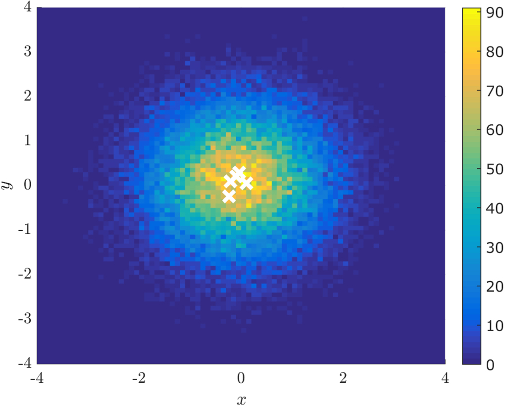
Here I present a numerical study to illustrate the proposal and confirm the theory. Assume an object that consists of 5 equally bright point sources with random positions within the square $-0.3\leqslant X\leqslant 0.3$ and $-0.3\leqslant Y\leqslant 0.3$. The average photon number is assumed to be $N=5\times 10\,000$ in total. Figure 2 shows an example of the generated source positions and a direct image with pixel size $\delta x\delta y=0.1\times 0.1$ and Poisson noise. I focus on the estimation of the first and second moments of the source distribution given by $\{{\theta }_{{\boldsymbol{\mu }}};{\boldsymbol{\mu }}=(1,0),(0,1),(2,0),(0,2),(1,1)\}$. For direct imaging, I use the estimator ${\check{\theta }}_{{\boldsymbol{\mu }}}={\boldsymbol{\mu }}!{\sum }_{j}{D}_{{\boldsymbol{\mu }}}({{\boldsymbol{r}}}_{j})m({{\boldsymbol{r}}}_{j})/N$, where $m({{\boldsymbol{r}}}_{j})$ is the photon count at a pixel positioned at ${{\boldsymbol{r}}}_{j}$. It can be shown that, in the small-pixel limit, this estimator is unbiased and approaches the CRB given by equation (4.8) for ${\rm{\Delta }}\ll 1$.

Zoom In Zoom Out Reset image size

For SPADE, I consider only the TEM₀₀, TEM₁₀, and TEM₀₁ modes, and the photons in all the other modes are discarded. As illustrated in figure 3, the iTEM1, iTEM2, and iTEM3 schemes suffice to estimate the parameters of interest. Table 2 lists the projections, and figure 4 plots the spatial wave functions for the projections. The light is assumed to be split equally among the three schemes, leading to 9 outputs; figure 5 shows a sample of the photon counts drawn from Poisson statistics. For the estimators, I use equations (4.12) and (4.16). Compared with the large number of pixels in direct imaging, the compressive nature of SPADE for moment estimation is an additional advantage.

Zoom In Zoom Out Reset image size

Zoom In Zoom Out Reset image size

Zoom In Zoom Out Reset image size

Table 2.  The projections for the SPADE measurement scheme depicted in figure 3. $| 0,0\rangle$ corresponds to the TEM₀₀ mode, $| 1,0\rangle$ corresponds to the TEM₁₀ mode, and $| 0,1\rangle$ corresponds to the TEM₀₁ mode.

iTEM1	iTEM2	iTEM3
$(| 0,0\rangle +| 1,0\rangle )/\sqrt{2}$	$(| 0,0\rangle +| 0,1\rangle )/\sqrt{2}$	$(| 1,0\rangle +| 0,1\rangle )/\sqrt{2}$
$(| 0,0\rangle -| 1,0\rangle )/\sqrt{2}$	$(| 0,0\rangle -| 0,1\rangle )/\sqrt{2}$	$(| 1,0\rangle -| 0,1\rangle )/\sqrt{2}$
$| 0,1\rangle$	$| 1,0\rangle$	$| 0,0\rangle$

Figure 6 plots the numerically computed mean-square errors (MSEs) for 100 randomly generated objects versus true parameters in log–log scale. Each error value for a given object is computed by averaging the squared difference between the estimator and the true parameter over 500 samples of Poissonian outputs. For comparison, figure 6 also plots the CRBs given by equations (4.8), (4.11), and (4.15), assuming ${{\rm{\Theta }}}_{{\boldsymbol{\mu }}}={\theta }_{{\boldsymbol{\mu }}}$ and neglecting the $O({\rm{\Delta }})$ term in equation (4.8). A few observations can be made:

• 1.  
  As shown by the plots in the first row of figure 6, SPADE is 3 times worse than direct imaging at estimating the first moments. This is because SPADE uses only 1/3 of the available photons to estimate each first moment.
• 2.  
  The theory suggests that the advantage of SPADE starts with the second moments, and indeed the other plots show that SPADE is substantially more precise at estimating them, even though SPADE uses only a fraction of the available photons to estimate each moment. This enhancement is a generalization of the recent results on two sources [1–6, 8, 9, 12–15].
• 3.  
  The errors are all remarkably tight to the CRBs, despite the simplicity of the estimators and the approximations in the bounds. In particular, the excellent performance of the SPADE estimator in the subdiffraction regime justifies its assumption of ${{\rm{\Theta }}}_{{\boldsymbol{\mu }}}={\theta }_{{\boldsymbol{\mu }}}$.

Zoom In Zoom Out Reset image size

In the diffraction-unlimited regime, it is not difficult to prove that direct imaging achieves the highest Fisher information allowed by quantum mechanics. To be precise, that regime can be defined as one in which the PSF is so sharp relative to the source distribution that $\{| {\psi }_{{\boldsymbol{R}}}\rangle ;{\boldsymbol{R}}\in \mathrm{supp}(F)\}$ can be approximated as the orthogonal position basis $\{| {\boldsymbol{r}}\rangle \}$. ${\rho }_{1}$ becomes diagonal in that basis, and the quantum Fisher information [1, 3, 43–46] is equal to the direct-imaging information given by equation (2.8). The physics in the opposite subdiffraction regime is entirely different, however, as diffraction causes $\{| {\psi }_{{\boldsymbol{R}}}\rangle \}$ to have significant overlaps with one another, and more judicious measurements can better deal with the resulting indistinguishability, as demonstrated in sections 4 and 5.

I now prove that SPADE is in fact near-quantum-optimal in estimating location and scale parameters of a source distribution in the subdiffraction regime. Suppose that the distribution has the form

$$\begin{eqnarray}&&F({\boldsymbol{R}}| \theta )=F({\boldsymbol{R}}({\boldsymbol{\xi }}| \theta )),\end{eqnarray} \tag{ 6.1 }$$

such that θ parameterizes a coordinate transformation ${\boldsymbol{R}}={\boldsymbol{R}}({\boldsymbol{\xi }}| \theta )$, and the transformation leads to a reference measure ${F}_{0}({\boldsymbol{\xi }})$ that is independent of θ. Taking ${\boldsymbol{R}}$ as a column vector, I can rewrite equation (2.2) as

$$\begin{eqnarray}&&{\rho }_{1}(\theta )={{\mathbb{E}}}_{0}(| {\psi }_{{\boldsymbol{R}}}\rangle \langle {\psi }_{{\boldsymbol{R}}}| ),\end{eqnarray} \tag{ 6.2 }$$

$$\begin{eqnarray}&&| {\psi }_{{\boldsymbol{R}}}\rangle ={{\rm{e}}}^{-{\rm{i}}{{\boldsymbol{k}}}^{\top }{\boldsymbol{R}}({\boldsymbol{\xi }}| \theta )}| {\psi }_{0}\rangle ,\end{eqnarray} \tag{ 6.3 }$$

where ${{\mathbb{E}}}_{0}(\cdot )\equiv \int {\rm{d}}{\boldsymbol{\xi }}{F}_{0}({\boldsymbol{\xi }})(\cdot )$ and ${\boldsymbol{k}}$ is the momentum operator in a column vector. I can now use the quantum upper bound on the Fisher information [1, 43, 46] and the convexity of the quantum Fisher information [69, 70] to prove that the Fisher information for any measurement is bounded as

$$\begin{eqnarray}&&J(\theta )\leqslant K({\rho }_{1}(\theta ))\leqslant \tilde{K}(\theta )\equiv N{{\mathbb{E}}}_{0}[K(| {\psi }_{{\boldsymbol{R}}}\rangle \langle {\psi }_{{\boldsymbol{R}}}| )],\end{eqnarray} \tag{ 6.4 }$$

where K is the quantum Fisher information proposed by Helstrom [44]. For the pure state, K can be computed analytically to give

$$\begin{eqnarray}&&K(| {\psi }_{{\boldsymbol{R}}}\rangle \langle {\psi }_{{\boldsymbol{R}}}| )=4\displaystyle \frac{\partial {{\boldsymbol{R}}}^{\top }({\boldsymbol{\xi }}| \theta )}{\partial {\theta }_{\mu }}\langle {\psi }_{0}| {\rm{\Delta }}{\boldsymbol{k}}{\rm{\Delta }}{{\boldsymbol{k}}}^{\top }| {\psi }_{0}\rangle \displaystyle \frac{\partial {\boldsymbol{R}}({\boldsymbol{\xi }}| \theta )}{\partial {\theta }_{\nu }},\end{eqnarray} \tag{ 6.5 }$$

$$\begin{eqnarray}&&{\rm{\Delta }}{\boldsymbol{k}}\equiv {\boldsymbol{k}}-\langle {\psi }_{0}| {\boldsymbol{k}}| {\psi }_{0}\rangle ,\end{eqnarray} \tag{ 6.6 }$$

leading to

$$\begin{eqnarray}&&{\tilde{K}}_{\mu \nu }=N{{\mathbb{E}}}_{0}\left[\displaystyle \frac{\partial {{\boldsymbol{R}}}^{\top }({\boldsymbol{\xi }}| \theta )}{\partial {\theta }_{\mu }}\displaystyle \frac{\partial {\boldsymbol{R}}({\boldsymbol{\xi }}| \theta )}{\partial {\theta }_{\nu }}\right]\end{eqnarray} \tag{ 6.7 }$$

for the gaussian PSF. For example, a location parameter can be expressed as ${\boldsymbol{R}}={\boldsymbol{\xi }}-(\theta ,0)$. Equation (6.7) then gives

$$\begin{eqnarray}&&\tilde{K}=N.\end{eqnarray} \tag{ 6.8 }$$

This can be attained by either direct imaging or iTEM1 in the subdiffraction regime.

The advantage of SPADE starts with the second moments, which are particularly relevant to scale estimation. Let ${\boldsymbol{R}}=\theta {\boldsymbol{\xi }}$, which results in

$$\begin{eqnarray}&&\tilde{K}=N{{\mathbb{E}}}_{0}({{\boldsymbol{\xi }}}^{\top }{\boldsymbol{\xi }}).\end{eqnarray} \tag{ 6.9 }$$

For the TEM measurement, on the other hand,

$$\begin{eqnarray}&&{p}^{({\rm{TEM}})}({\boldsymbol{q}}| \theta )={{\mathbb{E}}}_{0}\left({e}^{-{Q}_{X}}\displaystyle \frac{{Q}_{X}^{{q}_{x}}}{{q}_{x}!}{e}^{-{Q}_{Y}}\displaystyle \frac{{Q}_{Y}^{{q}_{y}}}{{q}_{y}!}\right),\end{eqnarray} \tag{ 6.10 }$$

$$\begin{eqnarray}&&{Q}_{X}\equiv \displaystyle \frac{{\theta }^{2}{\xi }_{X}^{2}}{4},\quad {Q}_{Y}\equiv \displaystyle \frac{{\theta }^{2}{\xi }_{Y}^{2}}{4}.\end{eqnarray} \tag{ 6.11 }$$

Defining

$$\begin{eqnarray}&&\bar{{\boldsymbol{q}}}\equiv \displaystyle \sum _{{\boldsymbol{q}}}{\boldsymbol{q}}{p}^{({\rm{TEM}})}({\boldsymbol{q}}| \theta )=\displaystyle \frac{{\theta }^{2}}{4}{{\mathbb{E}}}_{0}\left(\begin{array}{c}{\xi }_{X}^{2}\\ {\xi }_{Y}^{2}\end{array}\right),\end{eqnarray} \tag{ 6.12 }$$

$$\begin{eqnarray}&&{\boldsymbol{V}}\equiv \displaystyle \sum _{{\boldsymbol{q}}}({\boldsymbol{q}}-\bar{{\boldsymbol{q}}}){({\boldsymbol{q}}-\bar{{\boldsymbol{q}}})}^{\top }{p}^{({\rm{TEM}})}({\boldsymbol{q}}| \theta )\end{eqnarray} \tag{ 6.13 }$$

$$\begin{eqnarray}=\displaystyle \frac{{\theta }^{2}}{4}{{\mathbb{E}}}_{0}\left(\begin{array}{cc}{\xi }_{X}^{2} & 0\\ 0 & {\xi }_{Y}^{2}\end{array}\right)+O({\theta }^{4}),\end{eqnarray} \tag{ 6.14 }$$

and using the lower bound by Stein et al [71], I obtain

$$\begin{eqnarray}&&{J}^{({\rm{TEM}})}\geqslant N\displaystyle \frac{\partial {\bar{{\boldsymbol{q}}}}^{\top }}{\partial \theta }{{\boldsymbol{V}}}^{-1}\displaystyle \frac{\partial \bar{{\boldsymbol{q}}}}{\partial \theta }\to N{{\mathbb{E}}}_{0}({{\boldsymbol{\xi }}}^{\top }{\boldsymbol{\xi }}),\end{eqnarray} \tag{ 6.15 }$$

which approaches the quantum limit given by equation (6.9) for $\theta \to 0$. The argument can be made more precise if the form of ${F}_{0}({\boldsymbol{\xi }})$ is known, as the extended convexity of the quantum Fisher information can be used to obtain a tighter upper bound [70, 72], while the $O({\theta }^{4})$ term in equation (6.14) can be computed to obtain an explicit lower bound for any θ.

Though promising, the giant precision enhancements offered by SPADE do not imply unlimited imaging resolution for finite photon numbers. The higher moments are still more difficult to estimate even with SPADE in terms of the fractional error, which is $\sim {{\rm{CRB}}}_{{\boldsymbol{\mu }}{\boldsymbol{\mu }}}/{\theta }_{{\boldsymbol{\mu }}}^{2}=1/O(N{{\rm{\Delta }}}^{| {\boldsymbol{\mu }}{| }_{1}})$ for even $| {\boldsymbol{\mu }}{| }_{1}$ and $1/O(N{{\rm{\Delta }}}^{| {\boldsymbol{\mu }}{| }_{1}+1})$ for odd $| {\boldsymbol{\mu }}{| }_{1}$, meaning that more photons are needed to attain a desirable fractional error for higher-order moments. Intuitively, this is because of the inherent inefficiency of subdiffraction objects to couple to higher-order modes, and the need to accumulate enough photons in those modes to achieve an acceptable SNR. A related issue is the reconstruction of the full source distribution, which requires all moments in principle. A finite number of moments cannot determine the distribution uniquely by themselves [51], although a wide range of regularization methods, such as maximum entropy and basis pursuit, are available for more specific scenarios [51, 55, 57, 73, 74].

Despite these limitations, the fact remains that direct imaging is an even poorer choice of measurement for subdiffraction objects and SPADE can extract much more information, simply from the far field. For example, the size and shape of a star, a planetary system, a galaxy, or a fluorophore cluster that is poorly resolved under direct imaging can be identified much more accurately through the estimation of the second or higher moments by SPADE. Alternatively, SPADE can be used to reach a desirable precision with far fewer photons or a much smaller aperture, enhancing the speed or reducing the size of the imaging system for the more special purposes. In view of the statistical analysis in [2, 4, 6], the image-inversion interferometers proposed in [2, 4, 6, 23–25] are expected to be similarly useful for estimating the second moments. For larger objects, scanning in the manner of confocal microscopy [27] or adaptive alignment [1] should be helpful.

Many open problems remain; chief among them are the incorporation of prior information, generalizations for non-Gaussian PSFs, the derivation of more general quantum limits, the possibility of even better measurements, and experimental implementations. The quantum optimality of SPADE for general imaging is in particular an interesting question. These daunting problems may be attacked by more advanced methods in quantum metrology [43–46, 75–78], quantum state tomography [79–81], compressed sensing [55–57, 81], and photonics design [52–54].

Inspiring discussions with Ranjith Nair, Xiao-Ming Lu, Shan Zheng Ang, Shilin Ng, Laura Waller's group, Geoff Schiebinger, Ben Recht, and Alex Lvovsky are gratefully acknowledged. This work is supported by the Singapore National Research Foundation under NRF Grant No. NRF-NRFF2011-07 and the Singapore Ministry of Education Academic Research Fund Tier 1 Project R-263-000-C06-112.

Instead of assuming ${{\rm{\Theta }}}_{{\boldsymbol{\mu }}}={\theta }_{{\boldsymbol{\mu }}}$ as in section 4, I consider here the exact relation given by equation (3.6), which can be expressed as

$$\begin{eqnarray}&&{{\rm{\Theta }}}_{{\boldsymbol{\mu }}}={\theta }_{{\boldsymbol{\mu }}}-\displaystyle \frac{{\theta }_{{\boldsymbol{\mu }}+(\mathrm{2,0})}}{4}-\displaystyle \frac{{\theta }_{{\boldsymbol{\mu }}+(\mathrm{0,2})}}{4}-\ldots \end{eqnarray} \tag{ A1 }$$

For the TEM scheme, this implies that each ${\boldsymbol{q}}\mathrm{th}$ channel contains information about not only ${\theta }_{2{\boldsymbol{q}}}$ but also the higher-order moments. If I assume that each ${\boldsymbol{q}}\mathrm{th}$ channel is used to estimate only ${\theta }_{2{\boldsymbol{q}}}$, however, then the higher-order moments act only as nuisance parameters [59] to the estimation of ${\theta }_{2{\boldsymbol{q}}}$. This is a conservative assumption, as the data-processing inequality [42, 43] implies that neglecting outputs can only reduce the information, but the assumption also means that I do not need to consider any channel with order lower than ${\boldsymbol{q}}$ to compute the CRB with respect to ${\theta }_{2{\boldsymbol{q}}}$, simplifying the analysis below.

Given the above assumption, I can compute the information matrix with respect to the parameters $({\theta }_{2{\boldsymbol{q}}},{\theta }_{2{\boldsymbol{q}}+(\mathrm{2,0})},{\theta }_{2{\boldsymbol{q}}+(\mathrm{0,2})},\ldots )$ by considering only the ${\boldsymbol{q}}\mathrm{th}$ and higher-order channels; the result is

$$\begin{eqnarray}{J}^{({\rm{TEM}})}=\left(\begin{array}{ccc}{J}_{2{\boldsymbol{q}},2{\boldsymbol{q}}}^{({\rm{TEM}})} & {J}_{2{\boldsymbol{q}},2{\boldsymbol{q}}+(2,0)}^{({\rm{TEM}})} & \ldots \\ {J}_{2{\boldsymbol{q}}+(2,0),2{\boldsymbol{q}}}^{({\rm{TEM}})} & {J}_{2{\boldsymbol{q}}+(2,0),2{\boldsymbol{q}}+(2,0)}^{({\rm{TEM}})} & \ldots \\ \vdots & \vdots & \ddots \end{array}\right)\equiv {N}^{({\rm{TEM}})}\left(\begin{array}{cc}\alpha & {\eta }^{\top }\\ \eta & \gamma \end{array}\right),\end{eqnarray} \tag{ A2 }$$

where $\alpha =C({\boldsymbol{q}},{\boldsymbol{q}})/{{\rm{\Theta }}}_{2{\boldsymbol{q}}}$ and $\eta =O({{\rm{\Delta }}}^{-2| {\boldsymbol{q}}{| }_{1}})$ are determined only by the ${\boldsymbol{q}}\mathrm{th}$ channel, while $\gamma =O({{\rm{\Delta }}}^{-(2| {\boldsymbol{q}}{| }_{1}+2)})$ is mainly determined by the higher-order channels. The CRB with respect to ${\theta }_{2{\boldsymbol{q}}}$ becomes [59]

$$\begin{eqnarray}&&{{\rm{CRB}}}_{2{\boldsymbol{q}},2{\boldsymbol{q}}}^{({\rm{TEM}})}=\displaystyle \frac{1}{{N}^{({\rm{TEM}})}}{(\alpha -{\eta }^{\top }{\gamma }^{-1}\eta )}^{-1}.\end{eqnarray} \tag{ A3 }$$

The key here is that $\eta {\gamma }^{-1}{\eta }^{\top }=O({{\rm{\Delta }}}^{-2| {\boldsymbol{q}}{| }_{1}+2})$ is smaller than $\alpha =O({{\rm{\Delta }}}^{-2| {\boldsymbol{q}}{| }_{1}})$ by two orders of Δ, so

$$\begin{eqnarray}&&{{\rm{CRB}}}_{2{\boldsymbol{q}},2{\boldsymbol{q}}}^{({\rm{TEM}})}=\displaystyle \frac{1}{{N}^{({\rm{TEM}})}\alpha }[1+O({{\rm{\Delta }}}^{2})]\end{eqnarray} \tag{ A4 }$$

$$\begin{eqnarray}&&=\,\displaystyle \frac{{{\rm{\Theta }}}_{2{\boldsymbol{q}}}}{{N}^{({\rm{TEM}})}C({\boldsymbol{q}},{\boldsymbol{q}})}[1+O({{\rm{\Delta }}}^{2})]\end{eqnarray} \tag{ A5 }$$

$$\begin{eqnarray}&&=\,\displaystyle \frac{{\theta }_{2{\boldsymbol{q}}}}{{N}^{({\rm{TEM}})}C({\boldsymbol{q}},{\boldsymbol{q}})}[1+O({{\rm{\Delta }}}^{2})],\end{eqnarray} \tag{ A6 }$$

which is consistent with equation (4.11).

An intuitive way of understanding this result is to rewrite equation (A1) as

$$\begin{eqnarray}&&{\theta }_{{\boldsymbol{\mu }}}={{\rm{\Theta }}}_{{\boldsymbol{\mu }}}+\displaystyle \frac{{\theta }_{{\boldsymbol{\mu }}+(\mathrm{2,0})}}{4}+\displaystyle \frac{{\theta }_{{\boldsymbol{\mu }}+(\mathrm{0,2})}}{4}\,+\,\ldots ,\end{eqnarray} \tag{ A7 }$$

which implies that the total error in ${\theta }_{{\boldsymbol{\mu }}}$ consists of the error in ${{\rm{\Theta }}}_{{\boldsymbol{\mu }}}$ as well as the errors in the higher-order moments. The higher-order moments can be estimated much more accurately via the higher-order channels, so the effect of their uncertainties on the estimation of ${\theta }_{{\boldsymbol{\mu }}}$ is negligible. A similar exercise can be done for the iTEM schemes, with similar results.

In practice, such a careful treatment of the nuisance parameters is unlikely to be necessary in the subdiffraction regime, as the numerical analysis in section 5 shows that excellent results can be obtained simply by taking ${{\rm{\Theta }}}_{{\boldsymbol{\mu }}}={\theta }_{{\boldsymbol{\mu }}}$ without any correction.