Floquet perturbation theory: formalism and application to low-frequency limit

Floquet theorem is the statement that the solution to a differential equation with periodic coefficients can be written as a phase factor multiplied by a periodic function. A direct consequence of this statement in the condensed matter setting is the Bloch theorem for the solution to the Schrödinger equation in the presence of a spatially periodic potential due to a lattice. In our discussion, we reserve the Floquet theorem for a system with parameters that are periodic in time, t. The details of the Floquet theory formalism are presented in appendix A; here, we provide a summary.

For a Hamiltonian $\hat{H}(t)=\hat{H}(t+T)$ with period T = 2π/Ω, Floquet theorem states that the time-dependent Shrödinger equation ${\rm{i}}\tfrac{{\rm{d}}}{{\rm{d}}t}| \psi (t)\rangle =\hat{H}(t)| \psi (t)\rangle$ takes steady-state solutions of the form

$$\begin{eqnarray}&&| {\psi }_{\alpha }(t)\rangle ={{\rm{e}}}^{-{\rm{i}}{\epsilon }_{\alpha }t}| {\phi }_{\alpha }(t)\rangle ,\end{eqnarray} \tag{ 1 }$$

where the quasienergy _α is a conserved quantity and the periodic Floquet mode $| {\phi }_{\alpha }(t)\rangle =| {\phi }_{\alpha }(t+T)\rangle$ satisfies the Floquet Schrödinger equation

$$\begin{eqnarray}&&\left[\hat{H}(t)-{\rm{i}}\displaystyle \frac{{\rm{d}}}{{\rm{d}}t}\right]| {\phi }_{\alpha }(t)\rangle ={\epsilon }_{\alpha }| {\phi }_{\alpha }(t)\rangle .\end{eqnarray} \tag{ 2 }$$

The $| {\phi }_{\alpha }(t)\rangle$ form a time-dependent orthonormal basis for the Hilbert space ${\mathscr{H}}$ and can be viewed as the eigenstates of the time-dependent Floquet Hamiltonian $\hat{H}(t)-{\rm{i}}\tfrac{{\rm{d}}}{{\rm{d}}t}$ with time-independent eigenvalues belonging to the Floquet zone, ${\epsilon }_{\alpha }\in [-{\rm{\Omega }}/2,{\rm{\Omega }}/2]$. Using Floquet theorem, the evolution operator

$$\begin{eqnarray}&&\hat{U}(t,{t}_{0})={\rm{T}}{\rm{e}}{\rm{x}}{\rm{p}}\left[-{\rm{i}}{\int }_{{t}_{0}}^{t}\hat{H}(s){\rm{d}}s\right],\end{eqnarray} \tag{ 3 }$$

with t₀ < t and ${\rm{T}}{\rm{e}}{\rm{x}}{\rm{p}}$ the time-ordered exponential, can be decomposed as

$$\begin{eqnarray}&&\hat{U}(t,{t}_{0})=\hat{{\rm{\Phi }}}(t){{\rm{e}}}^{-{\rm{i}}(t-{t}_{0}){\hat{H}}_{F}}\hat{{\rm{\Phi }}}{({t}_{0})}^{\dagger },\end{eqnarray} \tag{ 4 }$$

where

$$\begin{eqnarray}&&{{\rm{e}}}^{-{\rm{i}}{t}{\hat{H}}_{F}}=\displaystyle \sum _{\alpha }{{\rm{e}}}^{-i{\epsilon }_{\alpha }t}| {\phi }_{\alpha }(0)\rangle \langle {\phi }_{\alpha }(0)| ,\end{eqnarray} \tag{ 5a }$$

$$\begin{eqnarray}&&\hat{{\rm{\Phi }}}(t)=\displaystyle \sum _{\alpha }| {\phi }_{\alpha }(t)\rangle \langle {\phi }_{\alpha }(0)| ,\end{eqnarray} \tag{ 5b }$$

define, respectively, the Floquet Hamiltonian ${\hat{H}}_{F}$ and the micromotion operator $\hat{{\rm{\Phi }}}(t)$. Here, we set $\hat{{\rm{\Phi }}}(0)=\hat{I}$. We could choose a different boundary condition by a change of basis to $| {\gamma }_{\alpha }\rangle ={\hat{{\rm{\Gamma }}}}^{\dagger }| {\phi }_{\alpha }(0)\rangle$, where $\hat{{\rm{\Gamma }}}$ is a unitary operator. In this basis, the Floquet Hamiltonian is ${\hat{{\rm{\Gamma }}}}^{\dagger }{\hat{H}}_{F}\hat{{\rm{\Gamma }}}$ and the micromotion operator ${\hat{{\rm{\Phi }}}}_{{\rm{\Gamma }}}(t)={\sum }_{\alpha }| {\phi }_{\alpha }(t)\rangle \langle {\gamma }_{\alpha }| =\hat{{\rm{\Phi }}}(t)\hat{{\rm{\Gamma }}}$, with ${\hat{{\rm{\Phi }}}}_{{\rm{\Gamma }}}(0)=\hat{{\rm{\Gamma }}}$. This freedom can lead to different truncated Floquet perturbative expansions, if $\hat{{\rm{\Gamma }}}$ depends on the perturbation parameter itself [33, 34]. We shall see an example of this in section 2.3. The evolution operator is independent of this choice.

The structure we have described above can be formalized in terms of an extended Floquet Hilbert space ${\mathscr{F}}={\mathscr{H}}\otimes {\mathscr{I}}$, where the auxiliary space ${\mathscr{I}}$ is the space of bounded periodic function over [0, T) [44]. We denote the states in ${\mathscr{H}},{\mathscr{I}},$ and ${\mathscr{F}}$ respectively by $| \cdot \rangle ,| \cdot ),$ and $| \cdot \rangle \,\rangle$ and the operators acting on each respective space as and $\hat{\hat{O}}$. The space ${\mathscr{I}}$ is spanned by a continuous orthonormal basis $\{| t)\},0\leqslant t\lt T$,

where is the identity operator in ${\mathscr{I}}$. The auxiliary space ${\mathscr{I}}$ is also spanned by the orthonormal Fourier basis

$$\begin{eqnarray}&&| n)={\int }_{0}^{T}{{\rm{e}}}^{-{\rm{i}}{n}{\rm{\Omega }}t}| t)\displaystyle \frac{{\rm{d}}t}{T},\quad n\in {\mathbb{Z}},\end{eqnarray} \tag{ 7 }$$

satisfying

We note

$$\begin{eqnarray}&&| t)=\displaystyle \sum _{n\in {\mathbb{Z}}}{{\rm{e}}}^{{\rm{i}}{n}{\rm{\Omega }}t}| n).\end{eqnarray} \tag{ 9 }$$

A loop in ${\mathscr{H}}$ is a one-parameter family of states $| \phi (t)\rangle$ that is cyclic, i.e. $| \phi (T)\rangle =| \phi (0)\rangle$. It can be lifted to a loop in ${\mathscr{F}}$ given by $| {\phi }_{t}\rangle \,\rangle := | \phi (t)\rangle | t)$. Associated with any loop $| {\phi }_{t}\rangle \,\rangle \in {\mathscr{F}}$ is the center of the loop,

$$\begin{eqnarray}&&| \overline{\phi }\rangle \,\rangle \equiv {\int }_{0}^{T}| {\phi }_{t}\rangle \,\rangle \displaystyle \frac{{\rm{d}}t}{T}.\end{eqnarray} \tag{ 10 }$$

We define the Fourier-integral and the time-derivative operators,

$$\begin{eqnarray}&&{\hat{\hat{\mu }}}_{n}=\hat{I}\otimes {\int }_{0}^{T}| t){{\rm{e}}}^{+{\rm{i}}{n}{\rm{\Omega }}t}(t| \displaystyle \frac{{\rm{d}}t}{T},\end{eqnarray} \tag{ 11a }$$

$$\begin{eqnarray}&&{\hat{\hat{Z}}}_{t}=\hat{I}\otimes \displaystyle \sum _{n\in {\mathbb{Z}}}| n)n{\rm{\Omega }}(n| ,\end{eqnarray} \tag{ 11b }$$

such that for a loop $| {\phi }_{t}\rangle \,\rangle \in {\mathscr{F}}$,

$$\begin{eqnarray}&&{\hat{\hat{\mu }}}_{n}| \overline{\phi }\rangle \,\rangle ={\int }_{0}^{T}{{\rm{e}}}^{+{\rm{i}}{n}{\rm{\Omega }}t}| {\phi }_{t}\rangle \,\rangle \displaystyle \frac{{\rm{d}}t}{T}\equiv | {\phi }_{n}\rangle \,\rangle ,\end{eqnarray} \tag{ 12 }$$

is the nth Fourier integral and

$$\begin{eqnarray}&&{\hat{\hat{Z}}}_{t}| \overline{\phi }\rangle \,\rangle ={\int }_{0}^{T}{\rm{i}}\displaystyle \frac{{\rm{d}}| \phi (t)\rangle }{{\rm{d}}t}| t)\displaystyle \frac{{\rm{d}}t}{T}\equiv {\rm{i}}| \overline{{\rm{d}}\phi /{\rm{d}}t}\rangle \,\rangle ,\end{eqnarray} \tag{ 13 }$$

is the center of the time-derivative of the loop. Then, the Floquet Schrödinger equation (2) can be written in ${\mathscr{F}}$ as

$$\begin{eqnarray}&&(\hat{\hat{H\,}}-{\hat{\hat{Z}}}_{t})| \overline{{\phi }_{\alpha }}\rangle \,\rangle ={\epsilon }_{\alpha }| \overline{{\phi }_{\alpha }}\rangle \,\rangle ,\end{eqnarray} \tag{ 14 }$$

where $\hat{\hat{H\,}}={\int }_{0}^{T}\hat{H}(t)\otimes | t)(t| \tfrac{{\rm{d}}t}{T}$.

Note, however, that the set $\{| \overline{{\phi }_{\alpha }}\rangle \,\rangle \}$ of solutions to equation (14) is not large enough to furnish a complete basis for ${\mathscr{F}}$. Noting that $[\hat{\hat{H}},{\hat{\hat{\mu }}}_{n}]=0$ and

$$\begin{eqnarray}&&[{\hat{\hat{\mu }}}_{n},{\hat{\hat{Z}}}_{t}]=n{\rm{\Omega }}{\hat{\hat{\mu }}}_{n},\end{eqnarray} \tag{ 15 }$$

we can write instead

$$\begin{eqnarray}&&(\hat{\hat{H\,}}-{\hat{\hat{Z}}}_{t})| {\phi }_{\alpha n}\rangle \,\rangle ={\epsilon }_{\alpha n}| {\phi }_{\alpha n}\rangle \,\rangle ,\end{eqnarray} \tag{ 16 }$$

where ${\epsilon }_{\alpha n}\equiv {\epsilon }_{\alpha }+n{\rm{\Omega }}$ and $| {\phi }_{\alpha n}\rangle \,\rangle \equiv {\hat{\hat{\mu }}}_{n}| \overline{{\phi }_{\alpha }}\rangle \,\rangle$. Indeed, ${\hat{\hat{\mu }}}_{n}$ is the ladder operator for $\hat{\hat{H\,}}-\hat{\hat{Z\,}}$, mapping the solution $| \overline{{\phi }_{\alpha }}\rangle \,\rangle$ with quasienergy ${\epsilon }_{\alpha }$ to $| {\phi }_{\alpha n}\rangle \,\rangle$ with quasienergy ${\epsilon }_{\alpha }+n{\rm{\Omega }}$. Now, the solutions $| {\phi }_{\alpha n}\rangle \,\rangle$ to equation (16) provide a full basis for ${\mathscr{F}}$.

Let us recap the Floquet perturbation theory [43] in the above language. The Floquet Schrödinger equation (16) can be inverted in ${\mathscr{F}}$ to give the Floquet Green's function

$$\begin{eqnarray}&&\hat{\hat{G\,}}(\epsilon )\equiv {(\epsilon -\hat{\hat{H}}+{\hat{\hat{Z}}}_{t})}^{-1}=\displaystyle \sum _{\alpha n}\displaystyle \frac{| {\phi }_{\alpha n}\rangle \,\rangle \langle \langle {\phi }_{\alpha n}| }{\epsilon -{\epsilon }_{\alpha }-n{\rm{\Omega }}}.\end{eqnarray} \tag{ 17 }$$

The Floquet Green's function can be employed to calculate a variety of responses of the driven system. In this work, we focus on its application to perturbation theory.

For the periodic Hamiltonian $\hat{H}(t)={\hat{H}}_{0}(t)+\hat{V}(t)$, where ${\hat{H}}_{0}(t)$ is the unperturbed Hamiltonian and $\hat{V}(t)$ is the perturbing potential (both having a common period T), we lift $\hat{H}(t)$ to $\hat{\hat{H}}={\hat{\hat{H}}}_{0}+\hat{\hat{V}}$ in ${\mathscr{F}}$. Paralleling the conventional time-independent perturbation expansion in ${\mathscr{F}}$, we then expand the solutions to the Floquet Schrödinger equation as

$$\begin{eqnarray}&&{\epsilon }_{\alpha }={\epsilon }_{\alpha (0)}+{\epsilon }_{\alpha (1)}+{\epsilon }_{\alpha (2)}\,+\,\cdots ,\end{eqnarray} \tag{ 18a }$$

$$\begin{eqnarray}&&| \overline{{\phi }_{\alpha }}\rangle \,\rangle =| \overline{{\phi }_{\alpha (0)}}\rangle \,\rangle +| \overline{{\phi }_{\alpha (1)}}\rangle \,\rangle +| \overline{{\phi }_{\alpha (2)}}\rangle \,\rangle +\cdots ,\end{eqnarray} \tag{ 18b }$$

with $({\hat{\hat{H}}}_{0}-\hat{\hat{Z}})| \overline{{\phi }_{\alpha (0)}}\rangle \,\rangle ={\epsilon }_{\alpha (0)}| \overline{{\phi }_{\alpha (0)}}\rangle \,\rangle$, to find for i ≥ 1,

$$\begin{eqnarray}&&{\epsilon }_{\alpha (i)}=\langle \,\langle \overline{{\phi }_{\alpha (0)}}| \hat{\hat{V\,}}| \overline{{\phi }_{\alpha (i-1)}}\rangle \,\rangle ,\end{eqnarray} \tag{ 19a }$$

$$\begin{eqnarray}&&| \overline{{\phi }_{\alpha (i)}}\rangle \,\rangle ={\hat{\hat{P}}}_{\alpha }{\hat{\hat{G}}}_{0\alpha }{\hat{\hat{P}}}_{\alpha }\left[\hat{\hat{V\,}}| \overline{{\phi }_{\alpha (i-1)}}\rangle \,\rangle -\displaystyle \sum _{j=1}^{i-1}{\epsilon }_{\alpha (i-j)}| \overline{{\phi }_{\alpha (j)}}\rangle \,\rangle \right],\end{eqnarray} \tag{ 19b }$$

where ${\hat{\hat{G}}}_{0\alpha }={({\epsilon }_{\alpha (0)}-{\hat{\hat{H}}}_{0}+{\hat{\hat{Z}}}_{t})}^{-1}$ is the Floquet Green's function for ${\hat{\hat{H}}}_{0}$, ${\hat{\hat{P}}}_{\alpha }=\hat{\hat{I}}-| \overline{{\phi }_{\alpha (0)}}\rangle \,\rangle \langle \,\langle \overline{{\phi }_{\alpha (0)}}|$ projects to the subspace of ${\mathscr{F}}$ that is orthogonal to $| \overline{{\phi }_{\alpha (0)}}\rangle \,\rangle$, and we have assumed the standard normalization $\langle \,\langle \overline{{\phi }_{\alpha (0)}}| \overline{{\phi }_{\alpha }}\rangle \,\rangle =1$.

Explicitly,

$$\begin{eqnarray}&&{\epsilon }_{\alpha (1)}={\int }_{0}^{T}\langle {\phi }_{\alpha (0)}(t)| \hat{V}(t)| {\phi }_{\alpha (0)}(t)\rangle \displaystyle \frac{{\rm{d}}t}{T},\end{eqnarray} \tag{ 20a }$$

$$\begin{eqnarray}&&| \overline{{\phi }_{\alpha (1)}}\rangle \,\rangle =\displaystyle \sum _{(\beta ,n)\ne (\alpha ,0)}\displaystyle \frac{\langle \,\langle {\phi }_{\beta n(0)}| \hat{\hat{V\,}}| \overline{{\phi }_{\alpha (0)}}\rangle \,\rangle }{{\epsilon }_{\alpha (0)}-{\epsilon }_{\beta (0)}-n{\rm{\Omega }}}| {\phi }_{\beta n(0)}\rangle \,\rangle ,\end{eqnarray} \tag{ 20b }$$

and

$$\begin{eqnarray}\begin{array}{rcl}{\epsilon }_{\alpha (2)} & = & \displaystyle \sum _{(\beta ,n)\ne (\alpha ,0)}\displaystyle \frac{| \langle \,\langle \overline{{\phi }_{\alpha (0)}}| \hat{\hat{V\,}}| {\phi }_{\beta n(0)}\rangle \,\rangle {| }^{2}}{{\epsilon }_{\alpha (0)}-{\epsilon }_{\beta (0)}-n{\rm{\Omega }}}\\ & = & \displaystyle \sum _{\begin{array}{c}n\ne 0\\ \beta \ne \alpha \end{array}}\displaystyle \frac{{\left|{\int }_{0}^{T}\langle {\phi }_{\alpha (0)}(t)| {{\rm{e}}}^{+{\rm{i}}{n}{\rm{\Omega }}t}\hat{V}(t)| {\phi }_{\beta (0)}(t)\rangle \tfrac{{\rm{d}}t}{T}\right|}^{2}}{{\epsilon }_{\alpha (0)}-{\epsilon }_{\beta (0)}-n{\rm{\Omega }}},\end{array}\end{eqnarray} \tag{ 21 }$$

etc.

As an example, we derive a high-frequency expansion using the Floquet perturbation theory (see [34] for a detailed discussion). Assuming the frequency is larger than the typical quasienergy, we shall take the unperturbed Hamiltonian ${\hat{\hat{H}}}_{0}=0$ and $\hat{\hat{V}}=\hat{\hat{H}}$. Therefore, _α(0) = 0, and $| \overline{{\phi }_{\alpha (0)}}\rangle \,\rangle$ can be obtained from lifting an arbitrary time-independent set $| {\phi }_{\alpha }\rangle$ in ${\mathscr{H}}$ to ${\mathscr{F}}$. Since the unperturbed quasienergies are degenerate for the same n, we employ degenerate perturbation theory, noting the matrix elements:

$$\begin{eqnarray}&&\langle \,\langle {\phi }_{\alpha n}| \hat{\hat{H\,}}| {\phi }_{\beta n}\rangle \,\rangle =\langle {\phi }_{\alpha }| {\hat{H}}^{(0)}| {\phi }_{\beta }\rangle ,\end{eqnarray} \tag{ 22 }$$

where the Fourier components are ${\hat{H}}^{(n)}={\int }_{0}^{T}{{\rm{e}}}^{{\rm{i}}{n}{\rm{\Omega }}t}\hat{H}(t)\tfrac{{\rm{d}}t}{T}$. Thus, at the lowest order, $| {\phi }_{\alpha }\rangle$ are chosen as the eigenstates of ${\hat{H}}^{(0)}$. After some algebra, using equations (20a), (20b), and (21), we find

$$\begin{eqnarray}&&{\epsilon }_{\alpha (1)}=\langle {\phi }_{\alpha }| {\hat{H}}^{(0)}| {\phi }_{\alpha }\rangle ,\end{eqnarray} \tag{ 23a }$$

$$\begin{eqnarray}&&{\epsilon }_{\alpha (2)}=\langle {\phi }_{\alpha }| \displaystyle \sum _{n\ne 0}\displaystyle \frac{[{\hat{H}}^{(-n)},{\hat{H}}^{(n)}]}{2n{\rm{\Omega }}}| {\phi }_{\alpha }\rangle ,\end{eqnarray} \tag{ 23b }$$

$$\begin{eqnarray}&&| {\phi }_{\alpha (1)}(t)\rangle =\displaystyle \sum _{n\ne 0}\displaystyle \frac{{\hat{H}}^{(-n)}{{\rm{e}}}^{{\rm{i}}{n}{\rm{\Omega }}t}}{n{\rm{\Omega }}}| {\phi }_{\alpha }\rangle .\end{eqnarray} \tag{ 23c }$$

Thus, in the basis $\{| {\phi }_{\alpha }\rangle \}$, the quasienergies are obtained by diagonalizing

$$\begin{eqnarray}&&{\hat{H}}_{F}\equiv {\hat{H}}^{(0)}+\displaystyle \sum _{n\ne 0}\displaystyle \frac{[{\hat{H}}^{(-n)},{\hat{H}}^{(n)}]}{2n{\rm{\Omega }}}+O(1/{{\rm{\Omega }}}^{2}),\end{eqnarray} \tag{ 24 }$$

and the micromotion takes the form

$$\begin{eqnarray}\begin{array}{rcl}\hat{{\rm{\Phi }}}(t) & = & \displaystyle \sum _{\alpha }| {\phi }_{\alpha }(t)\rangle \langle {\phi }_{\alpha }| \approx \hat{I}+\displaystyle \sum _{n\ne 0}\displaystyle \frac{{{\rm{e}}}^{{\rm{i}}{n}{\rm{\Omega }}t}}{n{\rm{\Omega }}}{\hat{H}}^{(-n)}\\ & \approx & \exp \left[{\rm{i}}\displaystyle \sum _{n\ne 0}\displaystyle \frac{{\hat{H}}^{(-n)}{{\rm{e}}}^{{\rm{i}}{n}{\rm{\Omega }}t}-{H}^{(n)}{{\rm{e}}}^{-{\rm{i}}{n}{\rm{\Omega }}t}}{2{\rm{i}}{n}{\rm{\Omega }}}\right].\end{array}\end{eqnarray} \tag{ 25 }$$

This is indeed the same expression obtained using other high-frequency expansions, such as van-Vleck perturbation theory [33–35]. We note that in this basis, the boundary condition $\hat{{\rm{\Phi }}}(0)=\hat{I}+{\sum }_{n\ne 0}{\hat{H}}^{(-n)}/(n{\rm{\Omega }})\ne \hat{I}$. Instead, ${\int }_{0}^{T}\mathrm{log}[\hat{{\rm{\Phi }}}(t)]\tfrac{{\rm{d}}t}{T}=0$, again in agreement with the van-Vleck theory.

We can restore the boundary condition to identity by the unitary transformation $\hat{{\rm{\Phi }}}(0)| {\phi }_{\alpha }\rangle =| {\phi }_{\alpha }(0)\rangle$ to the basis of perturbed Floquet modes. In this basis, we obtain

$$\begin{eqnarray}\begin{array}{rcl}{\hat{H}}_{F} & \mapsto & \hat{{\rm{\Phi }}}(0){\hat{H}}_{F}{\hat{{\rm{\Phi }}}}^{\dagger }(0)\\ & \approx & {\hat{H}}^{(0)}+\displaystyle \sum _{n\ne 0}\displaystyle \frac{[{\hat{H}}^{(-n)},{\hat{H}}^{(n)}]+[{\hat{H}}^{(0)},{\hat{H}}^{(n)}]+[{\hat{H}}^{(-n)},{\hat{H}}^{(0)}]}{2n{\rm{\Omega }}},\end{array}\end{eqnarray} \tag{ 26 }$$

and

$$\begin{eqnarray}\begin{array}{rcl}\hat{{\rm{\Phi }}}(t) & = & \displaystyle \sum _{\alpha }| {\phi }_{\alpha }(t)\rangle \langle {\phi }_{\alpha }(0)| \approx \hat{I}+\displaystyle \sum _{n\ne 0}\displaystyle \frac{{{\rm{e}}}^{{\rm{i}}{n}{\rm{\Omega }}t}-1}{n{\rm{\Omega }}}{\hat{H}}^{(-n)}\\ & \approx & \exp \left[{\rm{i}}\displaystyle \sum _{n\ne 0}\displaystyle \frac{{{\rm{e}}}^{{\rm{i}}{n}{\rm{\Omega }}t/2}{\hat{H}}^{(-n)}+{{\rm{e}}}^{-{\rm{i}}{n}{\rm{\Omega }}t/2}{\hat{H}}^{(n)}}{n{\rm{\Omega }}}\sin \displaystyle \frac{n{\rm{\Omega }}t}{2}\right].\end{array}\end{eqnarray} \tag{ 27 }$$

In the last step, we have written the micromotion in a form that is manifestly unitary. Note that now $\hat{{\rm{\Phi }}}(0)={\sum }_{\alpha }| {\phi }_{\alpha }(0)\rangle \langle {\phi }_{\alpha }(0)| =\hat{I}$ by orthonormality of the Floquet modes. This boundary condition and equations (26) and (27) agree with those obtained using the Floquet–Magnus expansion [33–35].

A perturbative expansion at low frequencies can be obtained by rescaling time to τ = Ωt and noting that the periodicity of the Hamiltonian $\hat{H}(\tau )$ is maintained when translating τ → τ + 2π. The Floquet Schrödinger equation in rescaled units read

$$\begin{eqnarray}&&(\hat{\hat{H\,}}-{\rm{\Omega }}{\hat{\hat{Z}}}_{\tau })| {\phi }_{\alpha n}\rangle \,\rangle ={\epsilon }_{\alpha n}| {\phi }_{\alpha n}\rangle \,\rangle ,\end{eqnarray} \tag{ 28 }$$

where the dimensionless ${\hat{\hat{Z}}}_{\tau }=\hat{I}\otimes {\sum }_{n}| n)n(n|$, and $\hat{\hat{H\,}}$ is defined below equation (14). One may now attempt a perturbative expansion at low frequencies taking $-{\rm{\Omega }}{\hat{\hat{Z}}}_{\tau }$ as the perturbation operator. However, there is a subtlety that must be addressed: the Floquet perturbation theory we developed in the previous section takes ${\hat{\hat{Z}}}_{\tau }$ as part of the unperturbed Hamiltonian. This is necessary to ensure that the eigenvalues of the unperturbed operator have the same modular structure as the final quasienergies; that is, if is a quasienergy obtained from the perturbative solution of equation (28), then  + nΩ for any $n\in {\mathbb{Z}}$ should also be a quasienergy solution of equation (28). By, taking $\hat{\hat{H\,}}$ as the unperturbed operator without including ${\hat{\hat{Z}}}_{\tau }$, the eigenvalues of the unperturbed Hamiltonian will no longer be modular. Indeed, the eigenstates of $\hat{\hat{H\,}}$ are nothing but the eigenstates of the instantaneous Hamiltonian $\hat{H}(\tau )$ lifted to ${\mathscr{F}}$:

$$\begin{eqnarray}&&\hat{\hat{H\,}}| {\psi }_{\alpha \tau }\rangle \,\rangle ={E}_{\alpha \tau }| {\psi }_{\alpha \tau }\rangle \,\rangle ,\end{eqnarray} \tag{ 29 }$$

where $| {\psi }_{\alpha \tau }\rangle \,\rangle =| {\psi }_{\alpha }(\tau )\rangle | \tau )$, $\hat{H}(\tau )| {\psi }_{\alpha }(\tau )\rangle ={E}_{\alpha }(\tau )| {\psi }_{\alpha }(\tau )\rangle$, and ${E}_{\alpha \tau }={E}_{\alpha }(\tau )$. The eigenvalues ${E}_{\alpha \tau }$ of $\hat{\hat{H\,}}$ are, therefore, not modular, unlike the eigenvalues ${\epsilon }_{\alpha n}$ of $\hat{\hat{H\,}}-{\rm{\Omega }}\hat{\hat{Z\,}}$. To avoid confusion, let us note that here τ is simply a label indexing the eigenvalues and eigenstates of $\hat{\hat{H\,}}$, even though the operator itself does not depend on a specific choice of this label.

Therefore, in order to use perturbation theory to build the spectrum of $\hat{\hat{H}}-{\rm{\Omega }}{\hat{\hat{Z}}}_{\tau }$ as a power series over the spectrum of $\hat{\hat{H}}$, we need to amend our Floquet perturbation theory to ensure we obtain a modular spectrum. This can be done by using the general relationship, employed in writing equation (16), between the modular Floquet spectrum and the Fourier integrals of the loop in ${\mathscr{F}}$ obtained by lifting the loop of Floquet modes in ${\mathscr{H}}$. Starting with the zeroth order solutions $| {\psi }_{\alpha \tau }\rangle \,\rangle$ in equation (29), we first use perturbation theory to find $| {\psi }_{\alpha \tau (i)}\rangle \,\rangle$ to the desired order i. The modular spectrum is then found by taking the Fourier transform of this loop in ${\mathscr{F}}$,

$$\begin{eqnarray}&&| {\phi }_{\alpha n(i)}\rangle \,\rangle ={\hat{\hat{\mu }}}_{n}| \overline{{\psi }_{\alpha (i)}}\rangle \,\rangle ={\int }_{0}^{2\pi }{{\rm{e}}}^{+{\rm{i}}{n}\tau }| {\psi }_{\alpha \tau (i)}\rangle \,\rangle {{\rm{d}}\!\!\!\!{-}}\tau ,\end{eqnarray} \tag{ 30 }$$

where ${{\rm{d}}\!\!\!\!{-}}\tau \equiv {\rm{d}}\tau /(2\pi )$. This defines the proper eigenstate of $\hat{\hat{H\,}}-{\rm{\Omega }}{\hat{\hat{Z}}}_{\tau }$ with a modular eigenvalue ${\epsilon }_{\alpha n(i)}={\epsilon }_{\alpha (i)}+n{\rm{\Omega }}$, and the quasienergy

$$\begin{eqnarray}&&{\epsilon }_{\alpha (i)}=\langle \,\langle \overline{{\phi }_{\alpha (0)}}| \hat{\hat{H\,}}| \overline{{\phi }_{\alpha (i)}}\rangle \,\rangle -{\rm{\Omega }}\langle \,\langle \overline{{\phi }_{\alpha (0)}}| \hat{\hat{Z\,}}| \overline{{\phi }_{\alpha (i-1)}}\rangle \,\rangle .\end{eqnarray} \tag{ 31 }$$

This equation follows from the Floquet Schrödinger equation and noting that $\langle \langle \overline{{\phi }_{\alpha (0)}}| \overline{{\phi }_{\alpha }}\rangle \,\rangle ={\int }_{0}^{2\pi }\langle \langle {\psi }_{\alpha \tau (0)}| {\psi }_{\alpha \tau }\rangle \,\rangle {{\rm{d}}\!\!\!\!{-}}\tau =1.$ Note that for i ≥ 1 the first term vanishes. Explicitly, for the first few terms we find,

$$\begin{eqnarray}&&{\epsilon }_{\alpha (0)}={\int }_{0}^{2\pi }{E}_{\alpha }(\tau ){{\rm{d}}\!\!\!\!{-}}\tau ;\end{eqnarray} \tag{ 32a }$$

$$\begin{eqnarray}&&{\epsilon }_{\alpha (1)}={\rm{\Omega }}{\int }_{0}^{2\pi }\langle {\psi }_{\alpha }(\tau )| \displaystyle \frac{1}{{\rm{i}}}\displaystyle \frac{\partial }{\partial \tau }| {\psi }_{\alpha }(\tau )\rangle {{\rm{d}}\!\!\!\!{-}}\tau ;\end{eqnarray} \tag{ 32b }$$

$$\begin{eqnarray}&&{\epsilon }_{\alpha (2)}={{\rm{\Omega }}}^{2}{\int }_{0}^{2\pi }\displaystyle \sum _{\beta \ne \alpha }\displaystyle \frac{{\left|\langle {\psi }_{\beta }| \tfrac{1}{{\rm{i}}}\tfrac{\partial }{\partial \tau }| {\psi }_{\alpha }\rangle \right|}^{2}}{{E}_{\alpha }(\tau )-{E}_{\beta }(\tau )}{{\rm{d}}\!\!\!\!{-}}\tau ;\end{eqnarray} \tag{ 32c }$$

and

$$\begin{eqnarray}&&| {\phi }_{\alpha n(1)}\rangle \,\rangle ={\rm{\Omega }}{\int }_{0}^{2\pi }\displaystyle \sum _{\beta \ne \alpha }\displaystyle \frac{\langle {\psi }_{\beta }| \tfrac{1}{{\rm{i}}}\tfrac{\partial }{\partial \tau }| {\psi }_{\alpha }\rangle }{{E}_{\alpha }(\tau )-{E}_{\beta }(\tau )}{{\rm{e}}}^{+{\rm{i}}{n}\tau }| {\psi }_{\beta \tau }\rangle \,\rangle {{\rm{d}}\!\!\!\!{-}}\tau .\end{eqnarray} \tag{ 33 }$$

There is one final loose end we now address: there is a gauge freedom in the choice of the instantaneous basis $| {\psi }_{\alpha }(\tau )\rangle$ that we need to fix. Explicitly, $| {\kappa }_{\alpha }(\tau )\rangle ={{\rm{e}}}^{-{\rm{i}}{{\rm{\Lambda }}}_{\alpha }(\tau )}| {\psi }_{\alpha }(\tau )\rangle$ with ${{\rm{\Lambda }}}_{\alpha }(2\pi )={{\rm{\Lambda }}}_{\alpha }(0)$ is another basis, satisfying

$$\begin{eqnarray}&&\begin{array}{l}\left[\hat{H}(\tau )-{\rm{i}}{\rm{\Omega }}\displaystyle \frac{\partial }{\partial \tau }\right]| {\kappa }_{\alpha }(\tau )\rangle =\left[{E}_{\alpha }(\tau )-{\rm{\Omega }}\displaystyle \frac{\partial {{\rm{\Lambda }}}_{\alpha }}{\partial \tau }\right]| {\kappa }_{\alpha }(\tau )\rangle -{\rm{i}}{\rm{\Omega }}{{\rm{e}}}^{-{\rm{i}}{{\rm{\Lambda }}}_{\alpha }(\tau )}\displaystyle \frac{\partial }{\partial \tau }| {\psi }_{\alpha }(\tau )\rangle .\end{array}\end{eqnarray} \tag{ 34 }$$

Thus, fixing the gauge by setting ${\rm{\Omega }}\partial {{\rm{\Lambda }}}_{\alpha }/\partial \tau ={E}_{\alpha }(\tau )-{\epsilon }_{\alpha (0)}$, that is,

$$\begin{eqnarray}&&{{\rm{\Lambda }}}_{\alpha }(\tau )=\displaystyle \frac{1}{{\rm{\Omega }}}{\int }_{0}^{\tau }[{E}_{\alpha }(s)-{\epsilon }_{\alpha (0)}]{\rm{d}}s,\end{eqnarray} \tag{ 35 }$$

up to a constant, we obtain

$$\begin{eqnarray}&&[\hat{H}(\tau )-{\rm{i}}{\rm{\Omega }}\displaystyle \frac{\partial }{\partial \tau }]| {\kappa }_{\alpha }(\tau )\rangle ={\epsilon }_{\alpha (0)}| {\kappa }_{\alpha }(\tau )\rangle +O({\rm{\Omega }}).\end{eqnarray} \tag{ 36 }$$

This is the zeroth-order Floquet Schrödinger equation⁴ . Therefore, we must indeed choose $| {\phi }_{\alpha (0)}\rangle \,\rangle =| \overline{{\kappa }_{\alpha }}\rangle \,\rangle$. This gauge-fixing was previously used by Martiskainen and Moiseyev [51]; however, they only justified its use numerically by showing that it improves the accuracy of the perturbative expansion. Here, we see that this gauge must be fixed for consistency of the adiabatic solution as the zeroth order term in the general low-frequency Floquet perturbation theory.

Our low-frequency expansion is obtained for periodically driven systems using Floquet perturbation theory. However, this same approach can be used for general non-periodic and slowly driven systems by treating the whole evolution as one long single cycle of a periodic drive. In this way, we can connect our results to other low-frequency approximations, such as the adiabatic perturbation theory [38–40] and the adiabatic-impulse theory [41, 42]. Our expressions obtained above for the evolution of the states are closely related to those obtained using the adiabatic perturbation theory [39, 40]. Our method is, however, simpler in its structure and casts the entire procedure in the language of time-independent perturbation theory in the extended Floquet Hilbert space. The adiabatic-impulse theory [41, 42], on the other hand, requires the identification of special points during the drive where Landau–Zener transitions are likely to occur. These points are then treated separately from the rest of the drive, which is taken to be adiabatic. The accuracy of this approach depends strongly on the specific shape of the drive and lacks a natural low-frequency perturbation parameter. In contrast, our approach, similar to the adiabatic perturbation theory, can be used for any drive protocol. Finally, the low-frequency Floquet perturbation theory formulated in this work naturally connects to other approximate methods for higher frequencies that also use the structure of the extended Floquet Hilbert space.

As an example, take the matrix Hamiltonian [52]

$$\begin{eqnarray}&&H(t)={\bf{B}}(t)\cdot {\boldsymbol{\sigma }},\end{eqnarray} \tag{ 37 }$$

of a spin-$\tfrac{1}{2}$ particle in a magnetic field ${\bf{B}}(t)$ rotating at frequency Ω and a fixed angle θ with the z-direction. (Here, ${\boldsymbol{\sigma }}$ is the vector of Pauli matrices and we set the magnetic moment to unity.) Taking ${\bf{n}}(t)=(\sin \theta \cos {\rm{\Omega }}t,\sin \theta \sin {\rm{\Omega }}t,\cos \theta )$ to be the unit vector in the direction of the magnetic field, and rescaling time as before to τ = Ωt, we have $H(\tau )=B{\bf{n}}(\tau )\cdot {\boldsymbol{\sigma }}$.

The exact solution to the Schrödinger equation is found by going to the rotating frame given by the periodic unitary transformation $S(\tau )={{\rm{e}}}^{{\rm{i}}\tau (1+{\sigma }_{z})/2}$, where the Hamiltonian is

$$\begin{eqnarray}\begin{array}{rcl}{H}_{\mathrm{rot}} & = & S(\tau )H(\tau ){S}^{\dagger }(t)-{\rm{i}}{\rm{\Omega }}S(\tau )\displaystyle \frac{{\rm{d}}}{{\rm{d}}\tau }{S}^{\dagger }(\tau )\\ & = & -\displaystyle \frac{{\rm{\Omega }}}{2}+B\sin \theta {\sigma }_{x}+\left(B\cos \theta -\displaystyle \frac{{\rm{\Omega }}}{2}\right){\sigma }_{z}.\end{array}\end{eqnarray} \tag{ 38 }$$

Since this is now time-independent, the solutions are found as the eigenstates $| {\chi }_{\pm }\rangle$ of H_rot with eigenvalues ${\epsilon }_{\pm }={{Be}}_{\pm }$, with ${e}_{\pm }=-({\rm{\Omega }}/2B)\pm \sqrt{{(\cos \theta -{\rm{\Omega }}/2B)}^{2}+{\sin }^{2}\theta }$. In the original frame, we find the Floquet steady states $| {\phi }_{\pm }(\tau )\rangle ={S}^{\dagger }(\tau )| {\chi }_{\pm }\rangle$ with eigenvalues _± as quasienergies. To compare these exact solutions with the low-frequency Floquet perturbation theory, we impose the normalization $\langle {\chi }_{\pm }({\rm{\Omega }})| {\chi }_{\pm }({\rm{\Omega }}=0)\rangle =1;$ then, the Fourier transform of the loop $| {\phi }_{\pm }(t)\rangle$ lifted to ${\mathscr{F}}$ reads

$$\begin{eqnarray}&&| {\phi }_{\pm n}\rangle \,\rangle =\left[\begin{array}{c}(\cos \theta \pm {e}_{\pm }){\delta }_{n,+1}\\ \sin \theta \,{\delta }_{n,0}\end{array}\right]\displaystyle \frac{| n)}{(1\pm {e}_{\pm }){f}_{\mp }(\theta /2)},\end{eqnarray} \tag{ 39 }$$

with ${f}_{+}(x)=\sin x$ and ${f}_{-}(x)=\cos x$. Expanding in powers of Ω, we find

$$\begin{eqnarray}&&{\epsilon }_{\pm (0)}=\pm B;\end{eqnarray} \tag{ 40a }$$

$$\begin{eqnarray}&&{\epsilon }_{\pm (1)}=-{\rm{\Omega }}{f}_{\mp }^{2}(\theta /2);\end{eqnarray} \tag{ 40b }$$

$$\begin{eqnarray}&&{\epsilon }_{\pm (2)}=\pm \displaystyle \frac{{{\rm{\Omega }}}^{2}}{8B}{\sin }^{2}\theta ,\quad \mathrm{etc};\end{eqnarray} \tag{ 40c }$$

$$\begin{eqnarray}&&| {\phi }_{\pm n(0)}\rangle \,\rangle =\left[\begin{array}{c}\pm {f}_{\mp }(\theta /2){\delta }_{n,+1}\\ {f}_{\pm }(\theta /2){\delta }_{n,0}\end{array}\right]| n);\end{eqnarray} \tag{ 40d }$$

$$\begin{eqnarray}&&| {\phi }_{\pm n(1)}\rangle \,\rangle =\displaystyle \frac{{\rm{\Omega }}\sin \theta }{4B}\left[\begin{array}{c}-{f}_{\pm }(\theta /2){\delta }_{n,+1}\\ \pm {f}_{\mp }(\theta /2){\delta }_{n,0}\end{array}\right]| n),\quad \mathrm{etc}.\end{eqnarray} \tag{ 40e }$$

The low-frequency Floquet perturbation series is based on the instantaneous spectrum of H(τ) of spin Pauli matrices along ${\bf{n}}(\tau )$, given by the eigenstates

$$\begin{eqnarray*}&&| {\psi }_{\pm }(\tau )\rangle =\left[\begin{array}{c}\pm {f}_{\mp }(\theta /2){{\rm{e}}}^{-{\rm{i}}\tau }\\ {f}_{\pm }(\theta /2)\end{array}\right]\end{eqnarray*}$$

with eigenvalues ${E}_{\pm }(\tau )=\pm B$. Since the instantaneous eigenvalues are time-independent, the gauge Λ_± = 0. Thus, at the lowest order, ${\epsilon }_{\pm (0)}={\int }_{0}^{2\pi }{E}_{\pm }(\tau ){{\rm{d}}\!\!\!\!{-}}\tau =\pm B$, and $| {\psi }_{\pm n(0)}\rangle \,\rangle ={\int }_{0}^{2\pi }{{\rm{e}}}^{+{\rm{i}}{n}\tau }| {\psi }_{\pm }(\tau )\rangle | \tau ){{\rm{d}}\!\!\!\!{-}}\tau$, which reproduce equations (40a) and (40d). Noting

$$\begin{eqnarray}&&\langle {\psi }_{\pm }(\tau )| \displaystyle \frac{1}{{\rm{i}}}\displaystyle \frac{\partial }{\partial \tau }| {\psi }_{\pm }(\tau )\rangle =-{f}_{\mp }^{2}(\theta /2),\end{eqnarray} \tag{ 41a }$$

$$\begin{eqnarray}&&\langle {\psi }_{+}(\tau )| \displaystyle \frac{1}{{\rm{i}}}\displaystyle \frac{\partial }{\partial \tau }| {\psi }_{-}(\tau )\rangle =\displaystyle \frac{1}{2}\sin \theta ,\end{eqnarray} \tag{ 41b }$$

and using equations (32b), (33), and (32c), we find precisely equations (40b), (40e), and (40c). Thus, our low-frequency Floquet perturbation theory yields just the same leading order terms as those obtained from the exact solution.

We shall now consider a more general periodic Hamiltonian $H(\tau )={\bf{d}}(\tau )\cdot {\boldsymbol{\sigma }}$, where ${\bf{d}}(\tau )=d(\tau ){\bf{n}}(\tau )$ is a vector, whose direction, ${\bf{n}}$, as well as its magnitude, d, change periodically in time. We denote the average ${\int }_{0}^{2\pi }d(\tau ){{\rm{d}}\!\!\!\!{-}}\tau \equiv \bar{d}$. Then, the Schrödinger equation is not, in general, exactly solvable. Transforming to the rotating frame, for example, will not produce a time-independent Hamiltonian any more. A high-frequency expansion can be developed in the rotating frame; however, this expansion fails at low enough frequency. Instead, we shall use the Floquet perturbation theory based on the instantaneous spectrum given by eigenstates $| {\psi }_{\pm }(\tau )\rangle ={{\rm{e}}}^{\mp {\rm{i}}{\rm{\Lambda }}(\tau )}\left[\begin{array}{c}\pm {f}_{\mp }(\theta (\tau )/2){{\rm{e}}}^{-{\rm{i}}\varphi (\tau )}\\ {f}_{\pm }(\theta (\tau )/2)\end{array}\right]$ and eigenvalues ${E}_{\pm }(\tau )=\pm d(\tau )$, where θ and φ are the polar angles of ${\bf{n}}$ and the gauge ${\rm{\Lambda }}(\tau )=\tfrac{1}{{\rm{\Omega }}}{\int }_{0}^{\tau }[d(s)-\bar{d}]{\rm{d}}s$. Now,

$$\begin{eqnarray}&&\langle {\psi }_{\pm }| \displaystyle \frac{1}{{\rm{i}}}\displaystyle \frac{\partial }{\partial \tau }| {\psi }_{\pm }\rangle =\displaystyle \frac{1\pm \cos \theta }{2}\displaystyle \frac{{\rm{d}}\varphi }{{\rm{d}}\tau },\end{eqnarray} \tag{ 42a }$$

$$\begin{eqnarray}&&\langle {\psi }_{-}| \displaystyle \frac{1}{{\rm{i}}}\displaystyle \frac{\partial }{\partial \tau }| {\psi }_{+}\rangle =\left(\displaystyle \frac{\sin \theta }{2}\displaystyle \frac{{\rm{d}}\varphi }{{\rm{d}}\tau }-\displaystyle \frac{{\rm{i}}}{2}\displaystyle \frac{{\rm{d}}\theta }{{\rm{d}}\tau }\right){{\rm{e}}}^{-2{\rm{i}}{\rm{\Lambda }}}.\end{eqnarray} \tag{ 42b }$$

So,

$$\begin{eqnarray}&&{\epsilon }_{\pm (0)}=\pm {\int }_{0}^{2\pi }d(\tau ){{\rm{d}}\!\!\!\!{-}}\tau =\pm \bar{d};\end{eqnarray} \tag{ 43a }$$

$$\begin{eqnarray}&&{\epsilon }_{\pm (1)}={\rm{\Omega }}{\int }_{0}^{2\pi }\displaystyle \frac{1\pm \cos \theta (\tau )}{2}\displaystyle \frac{{\rm{d}}\varphi }{{\rm{d}}\tau }{{\rm{d}}\!\!\!\!{-}}\tau ;\end{eqnarray} \tag{ 43b }$$

$$\begin{eqnarray}&&{\epsilon }_{\pm (2)}=\pm \displaystyle \frac{{{\rm{\Omega }}}^{2}}{8}{\int }_{0}^{2\pi }\displaystyle \frac{{\left(\tfrac{{\rm{d}}\varphi }{{\rm{d}}\tau }\right)}^{2}{\sin }^{2}\theta (\tau )+{\left(\tfrac{{\rm{d}}\theta }{{\rm{d}}\tau }\right)}^{2}}{d(\tau )}{{\rm{d}}\!\!\!\!{-}}\tau .\end{eqnarray} \tag{ 43c }$$

The first-order correction to the Floquet steady state reads

$$\begin{eqnarray}&&| {\psi }_{\pm (1)}(\tau )\rangle =\pm \displaystyle \frac{{\rm{\Omega }}}{2}\displaystyle \frac{\tfrac{{\rm{d}}\varphi }{{\rm{d}}\tau }\sin \theta \mp {\rm{i}}\tfrac{{\rm{d}}\theta }{{\rm{d}}\tau }}{d(\tau )}{{\rm{e}}}^{\mp 2{\rm{i}}{\rm{\Lambda }}(\tau )}| {\psi }_{\mp }(\tau )\rangle .\end{eqnarray} \tag{ 44 }$$

Consider the Hamiltonian

$$\begin{eqnarray}&&H(\tau )={af}(\tau ){\sigma }_{x}+b{\sigma }_{y},\end{eqnarray} \tag{ 45 }$$

where f(τ) is a periodic function satisfying $f(0)=-f(\pi )=1$ and a, b > 0. Half way during the cycle, the first term switches sign, thus realizing the usual situation in the Landau–Zener model for large frequencies. In our general notation, $H(\tau )=d(\tau ){\bf{n}}(\tau )\cdot {\boldsymbol{\sigma }}$, where $d(\tau )=\sqrt{{a}^{2}{f}^{2}(\tau )+{b}^{2}}$, θ = π/2, and $\cos \phi (\tau )={bf}(\tau )/d(\tau )$. The minimum gap in the instantaneous spectrum is b obtained when f vanishes. We take a ≫ b.

For b = 0, the exact solution for the evolution operator is $U(\tau )=\exp [-{\rm{i}}(a/{\rm{\Omega }})F(\tau ){\sigma }_{x}]$, where $F(\tau )={\int }_{0}^{\tau }f(s){\rm{d}}s$. Thus, the Floquet spectrum is given by the quasienergies ${\epsilon }_{\pm (0)}=\pm {aF}(2\pi )/(2\pi )=\pm {{af}}^{(0)}$ and Floquet steady states $| {\phi }_{\pm \tau (0)}\rangle \,\rangle =\tfrac{1}{\sqrt{2}}{[1\pm 1]}^{{\mathsf{T}}}{{\rm{e}}}^{\mp {\rm{i}}(a/{\rm{\Omega }}){\rm{\Lambda }}(\tau )}| \tau )$, with the micromotion phase ${\rm{\Lambda }}(\tau )=F(\tau )-{f}^{(0)}\tau$.

For b/Ω ≪ 1 or b/a ≪ 1, we expect the operator bσ_y to be 'small' compared to ${\hat{\hat{H}}}_{0}-{\rm{\Omega }}\hat{\hat{Z}}$ with ${H}_{0}(\tau )={af}(\tau ){\sigma }_{x};$ thus, we may use the Floquet perturbation theory in either the high-frequency limit Ω ≫ b or the high-amplitude limit a ≫ b to find corrections to the Floquet spectrum:

$$\begin{eqnarray}&&{\epsilon }_{\pm (1)}=0,\end{eqnarray} \tag{ 46a }$$

$$\begin{eqnarray}&&{\epsilon }_{\pm (2)}=\pm \displaystyle \frac{{b}^{2}}{{\rm{\Omega }}}\displaystyle \sum _{n}\displaystyle \frac{| {g}_{n}^{+}(2a/{\rm{\Omega }}){| }^{2}}{(2a/{\rm{\Omega }}){f}^{(0)}+n},\end{eqnarray} \tag{ 46b }$$

$$\begin{eqnarray}&&| \overline{{\phi }_{\pm (1)}}\rangle \,\rangle =\displaystyle \frac{b}{{\rm{\Omega }}}\displaystyle \sum _{n,m}\displaystyle \frac{{[{g}_{n}^{\pm }(2a/{\rm{\Omega }})]}^{* }{g}_{n-m}^{\pm }(a/{\rm{\Omega }})}{(2a/{\rm{\Omega }}){f}^{(0)}\pm n}\displaystyle \frac{1}{{\rm{i}}\sqrt{2}}\left[\begin{array}{c}1\\ \mp 1\end{array}\right]| m),\end{eqnarray} \tag{ 46c }$$

where ${g}_{n}^{\pm }(a/{\rm{\Omega }})={\int }_{0}^{2\pi }{{\rm{e}}}^{-{\rm{i}}{n}\tau }{{\rm{e}}}^{\pm {\rm{i}}(a/{\rm{\Omega }}){\rm{\Lambda }}(\tau )}{{\rm{d}}\!\!\!\!{-}}\tau$. Note that ${[{g}_{n}^{\pm }(a/{\rm{\Omega }})]}^{* }={g}_{-n}^{\mp }(a/{\rm{\Omega }})$. Thus, starting from an initial state $| {\phi }_{\pm (0)}(0)\rangle$, the probability of transitioning to state $| {\phi }_{\mp (0)}(\tau )\rangle$ at time τ is,

$$\begin{eqnarray}\begin{array}{rcl}{P}_{\pm }(\tau ) & = & {| \langle {\phi }_{\mp (0)}(\tau )| U(\tau )| {\phi }_{\pm (0)}(0)\rangle | }^{2}\\ & = & {\left|\displaystyle \sum _{\alpha }\langle {\phi }_{\mp (0)}(\tau )| {{\rm{e}}}^{-\tfrac{{\rm{i}}}{{\rm{\Omega }}}{\epsilon }_{\alpha }\tau }{\phi }_{\alpha }(\tau )\rangle \langle {\phi }_{\alpha }(0)| {\phi }_{\pm (0)}(0)\rangle \right|}^{2}\\ & \approx & | \langle {\phi }_{\mp (0)}(\tau )| {{\rm{e}}}^{-\tfrac{{\rm{i}}}{{\rm{\Omega }}}{\epsilon }_{\pm }\tau }{\phi }_{\pm (1)}(\tau )\rangle \langle {\phi }_{\pm (0)}(0)| {\phi }_{\pm (0)}(0)\rangle \\ & & +{\langle {\phi }_{\mp (0)}(\tau )| {{\rm{e}}}^{-\tfrac{{\rm{i}}}{{\rm{\Omega }}}{\epsilon }_{\mp }\tau }{\phi }_{\mp (0)}(\tau )\rangle \langle {\phi }_{\mp (1)}(0)| {\phi }_{\pm (0)}(0)\rangle | }^{2},\end{array}\end{eqnarray} \tag{ 47 }$$

where the approximation is to the second-order in b. This yields, after some algebra,

$$\begin{eqnarray}&&{P}_{\pm }(\tau )={\left|\displaystyle \frac{b}{{\rm{\Omega }}}{\int }_{0}^{\tau }{{\rm{e}}}^{\mp {\rm{i}}(2a/{\rm{\Omega }})F(s)}{\rm{d}}s\right|}^{2}.\end{eqnarray} \tag{ 48 }$$

This expression can also be obtained [53, 54] directly from the Schrödinger equation written in the adiabatic basis, $| \psi (\tau )\rangle ={\sum }_{\alpha =\pm }{A}_{\alpha }(\tau ){{\rm{e}}}^{-{\rm{i}}{\epsilon }_{\pm (0)}\tau /{\rm{\Omega }}}| {\phi }_{\alpha (0)}(\tau )\rangle$, which reads

$$\begin{eqnarray}&&\displaystyle \frac{{\rm{d}}{A}_{\pm }}{{\rm{d}}\tau }=\pm \displaystyle \frac{b}{{\rm{\Omega }}}{{\rm{e}}}^{\pm {\rm{i}}(2a/{\rm{\Omega }})F(\tau )}{A}_{\mp }(\tau ).\end{eqnarray} \tag{ 49 }$$

Starting with initial state $| {\phi }_{\pm (0)}(0)\rangle$ and assuming ${A}_{\pm }(\tau )=1+O(b/{\rm{\Omega }})$ during the evolution, we find ${A}_{\mp }(\tau )\approx \mp (b/{\rm{\Omega }}){\int }_{0}^{\tau }{{\rm{e}}}^{\mp {\rm{i}}(2a/{\rm{\Omega }})F(s)}{\rm{d}}s+O({b}^{2}/{{\rm{\Omega }}}^{2})$. Our derivation using the more systematic Floquet perturbation theory, apart from being an application of the formalism, shows that this result is valid not only when b/Ω ≪ 1, but also when b ≪ a, even for resonant b ≈ Ω/2 ≪ a. In the latter case, the usual rotating-wave approximation for large frequencies fails; however, the highly oscillating phase factor suppresses higher order corrections.

In figures 1 and 2, we compare ${P}_{-}(\tau )$ obtained by the exact numerical solution with the Floquet perturbation theory for $f(\tau )=\cos (\tau )$ as well as the sawtooth-linear function

$$\begin{eqnarray}f(\tau )=\left\{\begin{array}{ll}\tfrac{2}{\pi }\left(\tfrac{\pi }{2}-\tau \right) & 0\leqslant \tau \leqslant \pi ,\\ \tfrac{2}{\pi }\left(\tau -\tfrac{3\pi }{2}\right) & \pi \leqslant \tau \leqslant 2\pi .\end{array}\right.\end{eqnarray} \tag{ 50 }$$

Panels (a) and (b) in each figure show two choices of parameters at or near resonance b/Ω = 0.5. We note that while agreement is good in the first half of the cycle, it becomes less reliable in the second half. In fact, the end-of-cycle behavior of the Floquet perturbation theory is sensitive to the choice of parameters: for small final values of ${P}_{-}(\tau )$ around τ = 2π the agreement is reasonably good, but for certain larger final values, as in figure 2(b), the Floquet perturbation result becomes less reliable.

Zoom In Zoom Out Reset image size

Zoom In Zoom Out Reset image size

One way to understand these variations is to compare Floquet perturbation theory and exact results at half- and full-cycle. In panels (c) and (d) of each figure we compare our results for τ = π and τ = 2π, respectively, at a fixed ratio b/a ≪ 1 as a/Ω is varied. For the cosine ramp, the Floquet perturbation theory gives, ${P}_{-}(\pi )={\pi }^{2}{b}^{2}({[{{\bf{H}}}_{0}(2a/{\rm{\Omega }})]}^{2}+{[{J}_{0}(2a/{\rm{\Omega }})]}^{2}),$ and ${P}_{-}(2\pi )=4{\pi }^{2}{(b/{\rm{\Omega }})}^{2}{[{J}_{0}(2a/{\rm{\Omega }})]}^{2},$ where J₀ and ${{\bf{H}}}_{0}$ are, respectively, Bessel and Struve functions. For the linear ramp, we find ${P}_{-}(\pi )=[{F}_{-}^{2}(\sqrt{a/{\rm{\Omega }}})\,+{F}_{+}^{2}(\sqrt{a/{\rm{\Omega }}})]{\pi }^{2}{b}^{2}/(a{\rm{\Omega }})$ where ${F}_{\pm }(x)={\int }_{0}^{x}{f}_{\pm }(\pi {y}^{2}/2){\rm{d}}{y}$ are Fresnel integrals. We note that for large a/Ω ≫ 1, the prefactor approaches 1/2 and this reproduces the classic Landau–Zener–Stückelberg–Majorana formula [55–58],

$$\begin{eqnarray}&&{P}_{\mathrm{LZ}}=1-\exp [-{\pi }^{2}{b}^{2}/(2a{\rm{\Omega }})]\approx {\pi }^{2}{b}^{2}/(2a{\rm{\Omega }}).\end{eqnarray} \tag{ 51 }$$

However, the perturbative result starts to fail for larger a/Ω and fixed b/Ω since the magnitude of the exponent in P_LZ becomes large. We show P_LZ in panel (c) of each figure. We note that while the classic result is in very good agreement with the exact result, it misses the oscillations as a function of a/Ω. By contrast, the perturbative result captures these oscillations very well.

We also see the sporadic nature of the agreement between Floquet perturbation theory and the exact result in the second half-cycle. As seen in panels (d) of each figure, the final value ${P}_{-}(2\pi )$ shows large oscillations as a function of a/Ω and vanishes periodically. The Floquet perturbation theory result captures these oscillations and, in particular, the zeros of ${P}_{-}(2\pi )$ remarkably well. This feature is similar to the coherent destruction of transitions discussed in a periodically driven double-well potential [59–62]. For larger values of a/Ω going beyond its applicability, the Floquet perturbation theory overshoots the amplitude of the oscillations, eventually giving unphysical values larger than unity. This is due to the non-unitary nature of perturbative expansion of the micromotion operator. We expect that a more controlled expansion that respects the unitarity of the micromotion operator, similar to the Floquet–Magnus expansion, should resolve this problem.

First, let us say a few words about the different conventions for the range of quasienergies, which we formally restricted to the first Floquet zone $[-{\rm{\Omega }}/2,{\rm{\Omega }}/2]$. This choice is entirely arbitrary, of course, and it may be more suitable in some problems to make other choices. Shifting a quasienergy ${\epsilon }_{\alpha n}\mapsto {\epsilon }_{\alpha n}+m{\rm{\Omega }}$ maps $| {\phi }_{\alpha n}\rangle \,\rangle \mapsto {\hat{\hat{\mu }}}_{m}| {\phi }_{\alpha n}\rangle \,\rangle =| {\phi }_{\alpha n+m}\rangle \,\rangle$. Doing so for all or just a subset of quasienergies has no physical effect. For example, in equation (17) all such shifts can be absorbed into a shift of the summation variable n. Now, in Floquet perturbation theory, even if the unperturbed quasienergies _α(0) are in the first Floquet zone, the corrections, equation (19a), may not be. Thus, in this section, we shall relax this condition.

Degeneracies arise when two or more quasienergies ${\epsilon }_{\alpha }^{r}$, labeled by r, coincide when shifted by integer multiples of frequency, n^r. For accidental or symmetry related degeneracies, n^r = 0, and one might as well restrict the unperturbed quasienergies to the first Floquet zone from the outset. However, for low-frequency Floquet perturbation theory, where even the unperturbed quasienergies need to be calculated according to equation (32a), it is more convenient to allow unperturbed quasienergies take values outside the first Floquet zone. In this case, we shall assume the shifts n^r are unique. (Of course, one may always set one of them to zero.) For initially non-degenerate instantaneous energy eigenvalues ${E}_{\alpha }\ne {E}_{\beta }$, this happens only when the associated quasienergies become resonant at the Floquet zone center or edges; thus, ${\epsilon }_{\alpha }={\epsilon }_{\beta }+n{\rm{\Omega }}=m{\rm{\Omega }}/2$ for some integer m.

This is an unusual situation in textbook perturbation theory, since the zeroth-order quantities are resonant up to first order in the small quantity Ω. Nevertheless, we may still proceed by trying to find the proper superpositions of degenerate states that resolve the degeneracy. Define

$$\begin{eqnarray}&&| {\chi }_{\alpha }^{r}\rangle \,\rangle =\displaystyle \sum _{s}{c}_{\alpha }^{{rs}}{\hat{\hat{\mu }}}_{{n}^{r}}| \overline{{\phi }_{\alpha (0)}^{s}}\rangle \,\rangle ,\end{eqnarray} \tag{ 52 }$$

with coefficients ${c}_{\alpha }^{{rs}}$ to be determined by solving

$$\begin{eqnarray}&&(\hat{\hat{H\,}}-{\rm{\Omega }}\hat{\hat{Z\,}})| {\chi }_{\alpha }^{r}\rangle \,\rangle =(m{\rm{\Omega }}/2+{\epsilon }_{\alpha (1)}^{r})| {\chi }_{\alpha }^{r}\rangle \,\rangle +O({{\rm{\Omega }}}^{2}).\end{eqnarray} \tag{ 53 }$$

This yields,

$$\begin{eqnarray}&&\displaystyle \sum _{q}{W}_{\alpha }^{{rq}}{c}_{\alpha }^{{qs}}={\epsilon }_{\alpha (1)}^{s}{c}_{\alpha }^{{rs}},\end{eqnarray} \tag{ 54 }$$

where W_α is a matrix with diagonal elements ${W}_{\alpha }^{{rr}}={\epsilon }_{\alpha }^{r}+{n}^{r}{\rm{\Omega }}-m{\rm{\Omega }}/2$, and the off-diagonal elements,

$$\begin{eqnarray}\begin{array}{rcl}{W}_{\alpha }^{{rs}} & \equiv & -{\rm{\Omega }}\langle \,\langle \overline{{\phi }_{\alpha }^{r}}| {\hat{\hat{\mu }}}_{{n}^{r}}^{\dagger }\hat{\hat{Z}}{\hat{\hat{\mu }}}_{{n}^{s}}| \overline{{\phi }_{\alpha }^{s}}\rangle \,\rangle ,\quad r\ne s\\ & = & {\rm{\Omega }}{\displaystyle \int }_{0}^{2\pi }{{\rm{e}}}^{{\rm{i}}({n}_{s}-{n}_{r})\tau }\langle {\phi }_{\alpha }^{r}(\tau )| \displaystyle \frac{1}{{\rm{i}}}\displaystyle \frac{\partial }{\partial \tau }| {\phi }_{\alpha }^{s}(\tau )\rangle {{\rm{d}}\!\!\!\!{-}}\tau ,\end{array}\end{eqnarray} \tag{ 55 }$$

where we have used $\langle {\phi }_{\alpha }^{r}(\tau )| {\phi }_{\alpha }^{s}(\tau )\rangle =0$ for $r\ne s$. The eigenvalue set of equations in (54) constitute the first-order degenerate low-frequency Floquet perturbation theory.

Let us revisit the driven Landau–Zener model, equation (45), in the low-frequency Floquet perturbation theory. Here, we shall take $f(\tau )=\cos \tau$. The instantaneous eigenvalues are ${E}_{\pm }(\tau )=\pm \sqrt{{a}^{2}{\cos }^{2}\tau +{b}^{2}};$ so, the lowest-order quasienergies are

$$\begin{eqnarray}&&{\epsilon }_{\pm (0)}=\pm \displaystyle \frac{2b}{\pi }E(-{a}^{2}/{b}^{2}),\end{eqnarray} \tag{ 56a }$$

$$\begin{eqnarray}&&{\epsilon }_{\pm (2)}=\pm \displaystyle \frac{b}{4\pi }[E(-{a}^{2}/{b}^{2})-K(-{a}^{2}/{b}^{2})]{({\rm{\Omega }}/b)}^{2},\end{eqnarray} \tag{ 56b }$$

where E(x) and K(x) are complete elliptic integrals. (The first-order correction to quasienergy vanishes.) For Ω/b ≪ 1, one can always find quasienergy degeneracies by tuning a/b and sufficiently large shifts n. However, we note quasienergy degeneracies also occur for Ω/b ≳ 1, so the associated dynamics is not restricted to (very) low frequencies.

To the lowest order in Ω, the adiabatic solutions are

$$\begin{eqnarray}&&| \overline{{\phi }_{\pm (0)}}\rangle \,\rangle =\int \displaystyle \frac{{{\rm{e}}}^{\mp {\rm{i}}{\rm{\Lambda }}(\tau )}}{\sqrt{2}}\left[\begin{array}{c}{{\rm{e}}}^{-{\rm{i}}\varphi (\tau )}\\ \pm 1\end{array}\right]| \tau ){{\rm{d}}\!\!\!\!{-}}\tau ,\end{eqnarray} \tag{ 57 }$$

where $\cot \varphi (\tau )=(a/b)\cos \tau$ and the gauge ${\rm{\Lambda }}(\tau )=\tfrac{1}{{\rm{\Omega }}}{\int }_{0}^{\tau }[{E}_{+}(s)-{\epsilon }_{+(0)}]{\rm{d}}{s}$ can also be expressed in terms of an incomplete elliptical integral. Near a quasienergy degeneracy, ${\epsilon }_{+}=n{\rm{\Omega }}/2+{\rm{\Delta }}$ and ${\epsilon }_{-}=-n{\rm{\Omega }}/2-{\rm{\Delta }}$; thus, in the adiabatic basis $\{| \overline{{\phi }_{+(0)}}\rangle \,\rangle ,{\hat{\hat{\mu }}}_{n}| \overline{{\phi }_{-(0)}}\rangle \,\rangle \}$, m = n, and,

$$\begin{eqnarray}W=\left[\begin{array}{cc}{\rm{\Delta }} & {\rm{\Omega }}{z}_{n}^{* }\\ {\rm{\Omega }}{z}_{n} & -{\rm{\Delta }}\end{array}\right],\end{eqnarray} \tag{ 58 }$$

where ${z}_{n}=-\tfrac{1}{2}{\int }_{0}^{2\pi }({\rm{d}}\varphi /{\rm{d}}\tau ){{\rm{e}}}^{{\rm{i}}{n}\tau }{{\rm{e}}}^{2{\rm{i}}{\rm{\Lambda }}(\tau )}{{\rm{d}}\!\!\!\!{-}}\tau$ is nonzero only for odd n. We derive a closed-form expression for z_n in appendix B. Writing ${z}_{n}=-{\rm{i}}{\zeta }_{n}| {z}_{n}|$ with ${\zeta }_{n}=-\mathrm{sgn}(\mathrm{Im}\,{z}_{n})$, we find the solutions

$$\begin{eqnarray}&&| {\chi }^{+}\rangle \,\rangle =\cos \displaystyle \frac{{\theta }_{n}}{2}| \overline{{\phi }_{+(0)}}\rangle \,\rangle +{\rm{i}}{\zeta }_{n}\sin \displaystyle \frac{{\theta }_{n}}{2}{\hat{\hat{\mu }}}_{n}| \overline{{\phi }_{-(0)}}\rangle \,\rangle ,\end{eqnarray} \tag{ 59a }$$

$$\begin{eqnarray}&&| {\chi }^{-}\rangle \,\rangle =\sin \displaystyle \frac{{\theta }_{n}}{2}| \overline{{\phi }_{+(0)}}\rangle \,\rangle -{\rm{i}}{\zeta }_{n}\cos \displaystyle \frac{{\theta }_{n}}{2}{\hat{\hat{\mu }}}_{n}| \overline{{\phi }_{-(0)}}\rangle \,\rangle ,\end{eqnarray} \tag{ 59b }$$

with $0\lt {\theta }_{n}\lt \pi$ and $\tan {\theta }_{n}={\rm{\Omega }}| {z}_{n}| /{\rm{\Delta }}$. The quasienergy degeneracy is lifted to

$$\begin{eqnarray}&&{\epsilon }^{\pm }=+n{\rm{\Omega }}/2\pm \sqrt{{{\rm{\Delta }}}^{2}+| {z}_{n}{| }^{2}{{\rm{\Omega }}}^{2}}.\end{eqnarray} \tag{ 60 }$$

Exactly at the degeneracy, ${\epsilon }^{\pm }=+n{\rm{\Omega }}/2\pm {\rm{\Omega }}| {z}_{n}|$, θ_n = π/2, and $| {\chi }^{\pm }\rangle \,\rangle =\tfrac{1}{\sqrt{2}}({\hat{\hat{\mu }}}_{n}| \overline{{\phi }_{+(0)}}\rangle \,\rangle \pm {\rm{i}}{\zeta }_{n}| \overline{{\phi }_{-(0)}}\rangle \,\rangle )$.

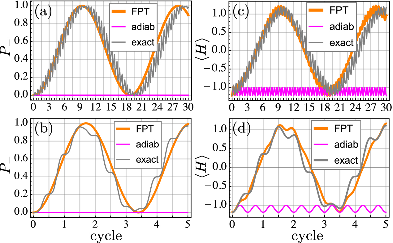
In figure 3, we show the transition probability and the expectation value of energy at two such quasienergy degeneracies, one at a lower frequency Ω/b = 0.75 and the other at a much higher frequency Ω/b = 2.45 with, respectively, n = 3 and n = 1. In both cases, we see that the low-frequency Floquet perturbation theory works well. This is remarkable for these frequencies are not particularly low compared to the minimum gap of $2b$. In fact, in the second case, the frequency Ω/b = 2.45 is larger than the gap, which is why it was chosen to obtain the lowest value of n = 1. In this case, numerically calculated quasienergies are far from Floquet zone edges and simply eyeballing their evolution with a/b does not hint at an avoided quasienergy degeneracy in the adiabatic approximation. Nevertheless, the lowest-order degenerate low-frequency Floquet perturbation theory produces a reasonably accurate result.

Zoom In Zoom Out Reset image size

A few remarks are in order. The low frequency oscillations observed in figure 3 are manifestations of Rabi-like oscillations between resonant states $| \overline{{\phi }_{+(0)}}\rangle \,\rangle$ and ${\hat{\hat{\mu }}}_{n}| \overline{{\phi }_{-(0)}}\rangle \,\rangle ;$ at degeneracy, the frequency of these oscillations is $| {z}_{n}| {\rm{\Omega }}$. These oscillations indicate a breakdown of adiabaticity [65, 45]: the system starting in the adiabatic state $| \overline{{\phi }_{-(0)}}\rangle \,\rangle$ would transition out fully over $1/(4| {z}_{n}| )$ cycles.

However, one must be quite careful about statements of adiabatic breakdown at low frequencies. For smooth drive protocols, the splitting $| {z}_{n}|$ is typically exponentially small at low frequencies, meaning that a non-adiabatic transition would take exponentially long times. For example, in appendix B we show that for Ω/b ≪ 1, a quasienergy degeneracy of the lowest shift order is obtained for a ∼ Ω with n ∼ bΩ and the quasienergy splitting vanishes as ${({\rm{\Omega }}/b)}^{2b/{\rm{\Omega }}}$. Thus, the transition time out of the adiabatic evolution diverges as a factorially large number $\sim {{\rm{e}}}^{-2(b/{\rm{\Omega }})\mathrm{log}(b/{\rm{\Omega }})}$. This trend is seen in figure 3. The period of Rabi oscillations is multiplied by a factor of about six when going from a principal resonance at n = 1 and Ω/b = 2.45 to the next resonance at n = 3 and Ω = 0.7. Using low-frequency Floquet perturbation theory, we found that for the first resonance in the driven Landau–Zener model with n = 7 and Ω/b = 0.29, this period rises up to more than 2 × 10⁵ cycles.

We have shown here that the celebrated adiabatic approximation is the lowest order of the more general low-frequency Floquet perturbation theory, which is built on the Floquet Green's function. The latter correctly accounts for corrections to the adiabatic approximation and, in particular, its potential breakdown due to Rabi oscillations at quasienergy degeneracies. We must note, too, that not all quasienergy resonances at low frequency exhibit Rabi oscillations. The low-frequency Floquet perturbation theory shows when adiabatic evolution is preserved due to protected quasienergy crossings. For example, in our driven Landau–Zener model, z_n = 0 for even n. At such crossings, Rabi oscillations become infinitely long, regardless of frequency, restoring adiabatic evolution in the degenerate subspace.

As a second application, we apply the (degenerate) low-frequency Floquet perturbation theory to a driven lattice model of non-interacting fermions, namely the SSH model. Both the static [66, 67] and driven [18, 46] versions of this model show distinct topological phases that are distinguished by the appearance of protected bound states at the edges of the lattice with open boundary conditions or a topological winding number in the Brillouin zone for a system with periodic boundary conditions.

The Hamiltonian for the SSH model is written as

$$\begin{eqnarray}&&\hat{H}=-\displaystyle \sum _{r=1}^{N-1}{w}_{r}{\hat{\xi }}_{r+1}^{\dagger }{\hat{\xi }}_{r}^{}+{\hat{H}}_{b}+{\rm{h}}.{\rm{c}}.,\end{eqnarray} \tag{ 61 }$$

where ${\hat{\xi }}_{r}^{\dagger }$ is the creation operator of a (spinless) fermion at site r, ${w}_{r}=w+{(-1)}^{r}\delta$ is the modulated hopping amplitude, and ${\hat{H}}_{b}$ is a boundary Hamiltonian that depends on the choice of boundary conditions. In the following we take w > 0 without loss of generality. For periodic boundary conditions, ${\hat{H}}_{b}={w}_{N}{\hat{\xi }}_{N}^{\dagger }{\hat{\xi }}_{1}^{}$, and even N we label the two-point unit cells with $s=\lfloor \tfrac{r+1}{2}\rfloor$, arrange the lattice operators into the spinor ${\hat{{\rm{\Xi }}}}_{s}^{\dagger }=({\hat{\xi }}_{r}^{\dagger },{\hat{\xi }}_{r+1}^{\dagger })$, and write the mode expansion ${\hat{{\rm{\Xi }}}}_{s}={\sum }_{s}{{\rm{e}}}^{{\rm{i}}{k}{s}}{\hat{{\rm{\Xi }}}}_{k}$ with lattice momentum $k\in [-\pi ,\pi ]$ to find $\hat{H}={\sum }_{k}{\hat{{\rm{\Xi }}}}_{k}^{\dagger }{h}_{k}^{}{\hat{{\rm{\Xi }}}}_{k}^{}$, with matrix Hamiltonian ${h}_{k}={{\bf{d}}}_{k}\cdot {\boldsymbol{\sigma }}$,

$$\begin{eqnarray}&&{d}_{{kx}}+{{\rm{i}}{d}}_{{ky}}\equiv {d}_{k}=2{{\rm{e}}}^{{\rm{i}}{k}/2}\left(w\cos \displaystyle \frac{k}{2}+{\rm{i}}\delta \sin \displaystyle \frac{k}{2}\right),\end{eqnarray} \tag{ 62 }$$

and energies ${E}_{k\pm }=\pm 2\sqrt{{w}^{2}{\cos }^{2}(k/2)+{\delta }^{2}{\sin }^{2}(k/2)}$. We also note that the Hamiltonian can be mapped unitarily to ${{\rm{e}}}^{{\rm{i}}\tfrac{k}{4}{\sigma }_{z}}{h}_{k}{{\rm{e}}}^{-{\rm{i}}\tfrac{k}{4}{\sigma }_{z}}=(w\cos \tfrac{k}{2}){\sigma }_{x}+(\delta \sin \tfrac{k}{2}){\sigma }_{y}$.

Now, we consider the driven SSH model, where δ(τ) is a periodic function of time with frequency Ω. We shall assume below that $| \delta | \leqslant w$ and denote the average $\bar{\delta }={\int }_{0}^{2\pi }\delta (\tau ){{\rm{d}}\!\!\!\!{-}}\tau$. In the low-frequency limit, to the lowest order in Ω, the adiabatic solutions are

$$\begin{eqnarray}&&| {\phi }_{k\pm (0)}(\tau )\rangle =\displaystyle \frac{{{\rm{e}}}^{\mp {\rm{i}}{{\rm{\Lambda }}}_{k}(\tau )-{\rm{i}}{k}{\sigma }_{z}/4}}{\sqrt{2}}\left[\begin{array}{c}{{\rm{e}}}^{{\rm{i}}{\varphi }_{k}(\tau )}\\ \pm 1\end{array}\right],\end{eqnarray} \tag{ 63 }$$

with ${{\rm{\Lambda }}}_{k}(\tau )=\tfrac{1}{{\rm{\Omega }}}{\int }_{0}^{\tau }[{E}_{k+}(s)-{\epsilon }_{k+(0)}]{\rm{d}}{s}$ and $\tan {\varphi }_{k}(\tau )=-[\delta (\tau )/w]\tan \tfrac{k}{2}$. The quasienergies in the leading-order non-degenerate low-frequency Floquet perturbation theory are ${\epsilon }_{k\pm }({\rm{\Omega }})={\epsilon }_{k\pm (0)}+{\epsilon }_{k\pm (1)}+{\epsilon }_{k\pm (2)}+\cdots$, where

$$\begin{eqnarray}&&{\epsilon }_{k\pm (0)}={\int }_{0}^{2\pi }{E}_{k\pm }(\tau ){{\rm{d}}\!\!\!\!{-}}\tau ,\end{eqnarray} \tag{ 64a }$$

$$\begin{eqnarray}&&{\epsilon }_{k\pm (1)}=0,\end{eqnarray} \tag{ 64b }$$

$$\begin{eqnarray}&&{\epsilon }_{k\pm (2)}=\displaystyle \frac{{{\rm{\Omega }}}^{2}}{8}{\int }_{0}^{2\pi }\displaystyle \frac{| \partial {\varphi }_{k}/\partial \tau {| }^{2}}{{E}_{k\pm }(\tau )}{{\rm{d}}\!\!\!\!{-}}\tau .\end{eqnarray} \tag{ 64c }$$

For a given ${\rm{\Omega }}\lt 4w$ there are a set of points $\pm {k}^{\wp }({\rm{\Omega }})$ in the Brillouin zone where quasienergies become degenerate: ${\epsilon }_{{k}^{\wp }+}={\epsilon }_{{k}^{\wp }-}+{n}_{{k}^{\wp }}{\rm{\Omega }}$, with $\lceil 4| \bar{\delta }| /{\rm{\Omega }}\rceil \leqslant {n}_{{k}^{\wp }}\leqslant \lfloor 4w/{\rm{\Omega }}\rfloor$. Near these points we must employ degenerate low-frequency Floquet perturbation theory. Expand ${\epsilon }_{k\pm }=\pm ({n}_{{k}^{\wp }}{\rm{\Omega }}/2+{{\rm{\Delta }}}_{k}^{\wp })$ and $| {\chi }_{k}^{\wp \pm }\rangle \,\rangle ={c}_{k+}^{\pm }| {\phi }_{k+(0)}\rangle \,\rangle +{c}_{k-}^{\pm }{\hat{\hat{\mu }}}_{{n}_{{k}^{\wp }}}| {\phi }_{k-(0)}\rangle \,\rangle$, to find ${W}_{k}^{\wp }\left[\begin{array}{c}{c}_{k+}^{\pm }\\ {c}_{k-}^{\pm }\end{array}\right]={\epsilon }_{k(1)}^{\wp \pm }\left[\begin{array}{c}{c}_{k+}^{\pm }\\ {c}_{k-}^{\pm }\end{array}\right]$ with ${W}_{k}^{\wp }=\left[\begin{array}{cc}{{\rm{\Delta }}}_{k}^{\wp } & {\rm{\Omega }}{z}_{k}^{\wp * }\\ {\rm{\Omega }}{z}_{k}^{\wp } & -{{\rm{\Delta }}}_{k}^{\wp }\end{array}\right]$. Here, ${z}_{k}^{\wp }\equiv {z}_{k,{n}_{{k}^{\wp }}}$, where

$$\begin{eqnarray}&&{z}_{k,n}=-\displaystyle \frac{1}{2}{\int }_{0}^{2\pi }{{\rm{e}}}^{{\rm{i}}{n}\tau }{{\rm{e}}}^{2{\rm{i}}{{\rm{\Lambda }}}_{k}(\tau )}\displaystyle \frac{\partial \varphi }{\partial \tau }{{\rm{d}}\!\!\!\!{-}}\tau ,\end{eqnarray} \tag{ 65 }$$

determines the gap opening at the degeneracy point as ${\epsilon }_{k(1)}^{\wp \pm }=\pm \sqrt{{{{\rm{\Delta }}}_{k}^{\wp }}^{2}+{{\rm{\Omega }}}^{2}| {z}_{k}^{\wp }{| }^{2}}$ and the solutions $| {\chi }_{k}^{\wp \pm }\rangle \,\rangle$ in a fashion similar to equation (59).

In figure 4 we compare the spectral measures obtained from the adiabatic approximation and the low-frequency Floquet perturbation theory with the numerically exact solution for a smooth drive protocol $\delta (\tau )=\bar{\delta }+{\delta }_{0}\cos \tau$. The quasienergies found using degenerate low-frequency Floquet perturbation theory match the exact solution remarkably well. The infidelity of an approximate solution, $| \phi (\tau )\rangle$, is defined as $1-{ \mathcal F }$, where ${ \mathcal F }(\tau )=| \langle {\phi }_{{\rm{e}}}(\tau )| \phi (\tau )\rangle {| }^{2}$ and $| {\phi }_{{\rm{e}}}(\tau )\rangle$ is the exact solution. Near a quasienergy degeneracy point, the infidelity of the adiabatic approximation increases dramatically as the frequency increases. The infidelity of the solution obtained using the degenerate low-frequency Floquet perturbation theory, on the other hand, is not only small relative to the adiabatic approximation, but it also remains small on the absolute scale even for larger frequencies. This demonstrates the consistency and accuracy of the Floquet perturbation theory.

Zoom In Zoom Out Reset image size

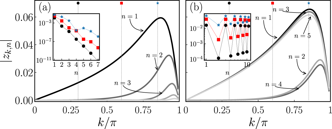
As the frequency is lowered, the order ${n}_{{k}^{\wp }}$ increases as $\sim 1/{\rm{\Omega }}$. For a smooth drive protocol, the adiabatic limit is obtained as the off-diagonal element ${z}_{k}^{\wp }$ vanishes. For example, for the sinusoidal drive protocol, ${z}_{k}^{\wp }$ vanishes exponentially similar to the Floquet resonances in the Landau–Zener model. However, for a drive protocol with sharp features, such as a step-wise protocol, the approach to the adiabatic limit may be slower or even violated. In figure 5 we show the dependence of ${z}_{k,n}$ on k and the order n of the quasienergy degeneracy. Indeed, as shown in figure 5(a) and the inset, for the sinusoidal drive protocol, ${z}_{k,n}$ vanishes with n in an exponential manner. However, for step-wise protocol, shown in figure 5(b), ${z}_{k,n}$ approaches a limiting value as n increases that depends on the parity of n.

Zoom In Zoom Out Reset image size

For a periodic Hamiltonian $\hat{H}(t)=\hat{H}(t+T)$, the full-period evolution operator, $\hat{U}(T)={T}{\rm{e}}{\rm{x}}{\rm{p}}\left[-{\rm{i}}{\int }_{0}^{T}\hat{H}(s){\rm{d}}s\right]$, is unitary and can be written as $\exp (-{\rm{i}}{T}{\hat{H}}_{F})$ for some Hermitian operator ${\hat{H}}_{F}$. The eigenvalues of $\hat{U}(T)$ are phases ${{\rm{e}}}^{-{\rm{i}}{\epsilon }_{\alpha }T}$ with eigenstates $| {\phi }_{\alpha }\rangle$,

$$\begin{eqnarray}&&\hat{U}(T)| {\phi }_{\alpha }\rangle ={{\rm{e}}}^{-{\rm{i}}{\epsilon }_{\alpha }T}| {\phi }_{\alpha }\rangle .\end{eqnarray} \tag{ A.1 }$$

Starting with a state $| {\psi }_{\alpha }(0)\rangle =| {\phi }_{\alpha }\rangle$, we have $| {\psi }_{\alpha }(T)\rangle =\hat{U}(T)| {\phi }_{\alpha }\rangle ={{\rm{e}}}^{-{\rm{i}}{\epsilon }_{\alpha }T}| {\phi }_{\alpha }\rangle$. Thus, defining $| {\phi }_{\alpha }(t)\rangle \equiv {{\rm{e}}}^{{\rm{i}}{\epsilon }_{\alpha }t}| {\psi }_{\alpha }(t)\rangle$, we find $| {\phi }_{\alpha }(T)\rangle =| {\phi }_{\alpha }\rangle \equiv | {\phi }_{\alpha }(0)\rangle$, i.e. $| {\phi }_{\alpha }(t)\rangle$ are periodic and $| {\psi }_{\alpha }(t)\rangle ={{\rm{e}}}^{-{\rm{i}}{\epsilon }_{\alpha }t}| {\phi }_{\alpha }(t)\rangle$. This is the Floquet theorem.

Since $\hat{U}(t)$ is unitary, it follows immediately that ${\epsilon }_{\alpha }\in {\mathbb{R}}$ and $\{| {\phi }_{\alpha }(0)\rangle \}$ is an orthonormal basis for ${\mathscr{H}}$. Therefore, the $| {\phi }_{\alpha }(t)\rangle ={{\rm{e}}}^{{\rm{i}}{\epsilon }_{\alpha }t}\hat{U}(t)| {\phi }_{\alpha }(0)\rangle$ also form an orthonormal basis for ${\mathscr{H}}$. Since the quasienergies are modular, defined only through the eigenvalues ${{\rm{e}}}^{-{\rm{i}}{\epsilon }_{\alpha }T}$ of $\hat{U}(T)$, we may restrict them to be in the first Floquet zone, ${\epsilon }_{\alpha }\in [-{\rm{\Omega }}/2,{\rm{\Omega }}/2]$. Using this structure, the evolution operator is completely defined by its action $\hat{U}(t)| {\phi }_{\alpha }(0)\rangle ={{\rm{e}}}^{-{\rm{i}}{\epsilon }_{\alpha }t}| {\phi }_{\alpha }(t)\rangle ;$ thus,

$$\begin{eqnarray}&&\hat{U}(t)=\displaystyle \sum _{\alpha }{{\rm{e}}}^{-{\rm{i}}{\epsilon }_{\alpha }t}| {\phi }_{\alpha }(t)\rangle \langle {\phi }_{\alpha }(0)| =: \hat{{\rm{\Phi }}}(t){{\rm{e}}}^{-{\rm{i}}{t}{\hat{H}}_{F}},\end{eqnarray} \tag{ A.2 }$$

where the sum over α is understood as an integral whenever α is continuous, and

$$\begin{eqnarray}&&\hat{{\rm{\Phi }}}(t)=\displaystyle \sum _{\alpha }| {\phi }_{\alpha }(t)\rangle \langle {\phi }_{\alpha }(0)| ,\end{eqnarray} \tag{ A.3 }$$

$$\begin{eqnarray}&&{{\rm{e}}}^{-{\rm{i}}{t}{\hat{H}}_{F}}=\displaystyle \sum _{\alpha }{{\rm{e}}}^{-{\rm{i}}{t}{\epsilon }_{\alpha }}| {\phi }_{\alpha }(0)\rangle \langle {\phi }_{\alpha }(0)| .\end{eqnarray} \tag{ A.4 }$$

Here $\hat{{\rm{\Phi }}}(t)=\hat{{\rm{\Phi }}}(t+T)$ is a unitary periodic operator, with the boundary condition $\hat{{\rm{\Phi }}}(0)=\hat{I}$, called the micromotion operator. It produces the periodic evolution of the Floquet modes, $| {\phi }_{\alpha }(t)\rangle =\hat{{\rm{\Phi }}}(t)| {\phi }_{\alpha }(0)\rangle$. The time-independent, Hermitian operator ${\hat{H}}_{F}$ is called the Floquet Hamiltonian.

In the above decomposition, we chose to set the initial time t₀ = 0. This choice is arbitrary; we could choose any other time within a cycle $0\leqslant {t}_{0}\lt T$. In general, for t > t₀ we have:

$$\begin{eqnarray}&&\hat{U}(t,{t}_{0})={T}{\rm{e}}{\rm{x}}{\rm{p}}\left[-{\rm{i}}{\int }_{{t}_{0}}^{t}\hat{H}(s){\rm{d}}s\right]\end{eqnarray} \tag{ A.5 }$$

$$\begin{eqnarray}&&=\displaystyle \sum _{\alpha }{{\rm{e}}}^{-{\rm{i}}{\epsilon }_{\alpha }(t-{t}_{0})}| {\phi }_{\alpha }(t)\rangle \langle {\phi }_{\alpha }({t}_{0})| \end{eqnarray} \tag{ A.6 }$$

$$\begin{eqnarray}&&=\hat{{\rm{\Phi }}}(t,{t}_{0}){{\rm{e}}}^{-{\rm{i}}(t-{t}_{0}){\hat{H}}_{F}({t}_{0})}\end{eqnarray} \tag{ A.7 }$$

$$\begin{eqnarray}&&={{\rm{e}}}^{-{\rm{i}}(t-{t}_{0}){\hat{H}}_{F}(t)}\hat{{\rm{\Phi }}}(t,{t}_{0}),\end{eqnarray} \tag{ A.8 }$$

where

$$\begin{eqnarray}&&\hat{{\rm{\Phi }}}(t,{t}_{0})=\displaystyle \sum _{\alpha }| {\phi }_{\alpha }(t)\rangle \langle {\phi }_{\alpha }({t}_{0})| =\hat{{\rm{\Phi }}}(t)\hat{{\rm{\Phi }}}{({t}_{0})}^{\dagger },\end{eqnarray} \tag{ A.9 }$$

$$\begin{eqnarray}\begin{array}{rcl}{{\rm{e}}}^{-{\rm{i}}{s}{\hat{H}}_{F}({t}_{0})} & = & \displaystyle \sum _{\alpha }{{\rm{e}}}^{-{\rm{i}}{s}{\epsilon }_{\alpha }}| {\phi }_{\alpha }({t}_{0})\rangle \langle {\phi }_{\alpha }({t}_{0})| \\ & = & \hat{{\rm{\Phi }}}({t}_{0}){{\rm{e}}}^{-{\rm{i}}{s}{\hat{H}}_{F}}\hat{{\rm{\Phi }}}{({t}_{0})}^{\dagger }.\end{array}\end{eqnarray} \tag{ A.10 }$$

The two-time micromotion operator produces the periodic evolution of Floquet modes, $\hat{{\rm{\Phi }}}(t,{t}_{0})| {\phi }_{\alpha }({t}_{0})\rangle =| {\phi }_{\alpha }(t)\rangle$.

We note that, since $\left[\hat{H}(t)-{\rm{i}}\tfrac{{\rm{d}}}{{\rm{d}}t}\right]| {\phi }_{\alpha }(t)\rangle ={\epsilon }_{\alpha }| {\phi }_{\alpha }(t)\rangle$, the time-dependent Floquet Hamiltonian can be resolved as

$$\begin{eqnarray}&&\hat{H}(t)-{\rm{i}}\displaystyle \frac{{\rm{d}}}{{\rm{d}}t}=\displaystyle \sum _{\alpha }{\epsilon }_{\alpha }| {\phi }_{\alpha }(t)\rangle \langle {\phi }_{\alpha }(t)| \equiv {\hat{H}}_{F}(t).\end{eqnarray} \tag{ A.11 }$$

Moreover, ${\hat{H}}_{F}$ and ${\hat{H}}_{F}({t}_{0})$ are unitarily equivalent. Especially, the eigenvalues of ${\hat{H}}_{F}({t}_{0})$ do not depend on the initial time. However, when certain approximate methods are used to find ${\hat{H}}_{F}({t}_{0})$ it turns out the eigenvalues acquire a spurious dependence on t₀. One way to avoid this problem is by using the decomposition $\hat{{\rm{\Phi }}}(t,{t}_{0})=\hat{{\rm{\Phi }}}(t)\hat{{\rm{\Phi }}}{({t}_{0})}^{\dagger }$ to write

$$\begin{eqnarray}&&\hat{U}(t,{t}_{0})=\hat{{\rm{\Phi }}}(t){{\rm{e}}}^{-{\rm{i}}(t-{t}_{0}){\hat{H}}_{F}}\hat{{\rm{\Phi }}}{({t}_{0})}^{\dagger }.\end{eqnarray} \tag{ A.12 }$$

The dependence on t₀ is then entirely accounted for in the micromotion operator.

The structure we have described in the previous section can be formalized in terms of an extended Floquet Hilbert space ${\mathscr{F}}={\mathscr{H}}\otimes {\mathscr{I}}$, where the auxiliary space ${\mathscr{I}}$ is the space of bounded periodic function over [0, T). It is spanned by a continuous orthonormal basis $\{| t)\},0\leqslant t\lt T$,

$$\begin{eqnarray}&&(t^{\prime} | t)=T\delta (t-t^{\prime} ),\end{eqnarray} \tag{ A.13 }$$

Here, is the identity operator in ${\mathscr{I}}$. Equivalently, it is also spanned by the orthonormal Fourier basis

$$\begin{eqnarray}&&| n)={\int }_{0}^{T}{{\rm{e}}}^{-{\rm{i}}{n}{\rm{\Omega }}t}| t)\displaystyle \frac{{\rm{d}}t}{T},\quad n\in {\mathbb{Z}},\end{eqnarray} \tag{ A.15 }$$

which satisfy

$$\begin{eqnarray}&&(n| m)={\delta }_{{nm}},\end{eqnarray} \tag{ A.16 }$$

Using the Poisson summation formula, ${\sum }_{n\in {\mathbb{Z}}}{{\rm{e}}}^{{\rm{i}}{n}{\rm{\Omega }}t}=T{\sum }_{p\in {\mathbb{Z}}}\delta (t-{pT})$, these relations can be inverted to give

$$\begin{eqnarray}&&| t)=\displaystyle \sum _{n\in {\mathbb{Z}}}{{\rm{e}}}^{{\rm{i}}{n}{\rm{\Omega }}t}| n).\end{eqnarray} \tag{ A.18 }$$

Note that if we extended the range of t to ${\mathbb{R}}$ periodically by defining $| t+T)=| t)$, then

Now, a loop in ${\mathscr{H}}$ given by the one-parameter family of states $| \phi (t)\rangle$, with $| \phi (T)\rangle =| \phi (0)\rangle$, can be lifted to a loop in ${\mathscr{F}}$ given by $| {\phi }_{t}\rangle \,\rangle := | \phi (t)\rangle | t)$. Associated with any loop in ${\mathscr{F}}$ is the center

$$\begin{eqnarray}&&| \overline{\phi }\rangle \,\rangle := {\int }_{0}^{T}| {\phi }_{t}\rangle \,\rangle \displaystyle \frac{{\rm{d}}t}{T}.\end{eqnarray} \tag{ A.20 }$$

From the center of a lifted loop in ${\mathscr{F}}$ one can in turn obtain the corresponding loop in ${\mathscr{H}}$ by the projection

$$\begin{eqnarray}&&| \phi (t)\rangle =(t| \overline{\phi }\rangle \,\rangle .\end{eqnarray} \tag{ A.21 }$$

We also note that $| \overline{\phi }\rangle \,\rangle ={\sum }_{n\in {\mathbb{Z}}}| {\phi }^{(n)}\rangle | n),$ where the Fourier components

$$\begin{eqnarray}&&| {\phi }^{(n)}\rangle ={\int }_{0}^{T}{{\rm{e}}}^{+{\rm{i}}{n}{\rm{\Omega }}t}| \phi (t)\rangle \displaystyle \frac{{\rm{d}}t}{T}.\end{eqnarray} \tag{ A.22 }$$

Similarly, a two-parameter periodic family of operators $\hat{A}(t,t^{\prime} )\,:{\mathscr{H}}\to {\mathscr{H}}$ with $\hat{A}(t+T,t^{\prime} )=\hat{A}(t,t^{\prime} +T)=\hat{A}(t,t^{\prime} )$ is lifted to an operator $\hat{\hat{A\,}}\,:{\mathscr{F}}\to {\mathscr{F}}$ defined as

$$\begin{eqnarray}&&\hat{\hat{A}}={\int }_{0}^{T}| t)\hat{A}(t,t^{\prime} )(t^{\prime} | \displaystyle \frac{{\rm{d}}t}{T}\displaystyle \frac{{\rm{d}}t^{\prime} }{T}=\displaystyle \sum _{n,n^{\prime} \in {\mathbb{Z}}}| n){\hat{A}}^{(n,n^{\prime} )}(n^{\prime} | ,\end{eqnarray} \tag{ A.23 }$$

with

$$\begin{eqnarray}&&{\hat{A}}^{(n,n^{\prime} )}={\int }_{0}^{T}{{\rm{e}}}^{{\rm{i}}{n}{\rm{\Omega }}t}{{\rm{e}}}^{-{\rm{i}}{n}^{\prime} {\rm{\Omega }}t^{\prime} }\hat{A}(t,t^{\prime} )\displaystyle \frac{{\rm{d}}t}{T}\displaystyle \frac{{\rm{d}}t^{\prime} }{T}.\end{eqnarray} \tag{ A.24 }$$

Two special cases arise when $\hat{\hat{A\,}}$ is diagonal in either ${\mathscr{I}}$ or ${\mathscr{H}}$. As an example of the former case, and ${\hat{A}}^{(n,n^{\prime} )}={\hat{A}}^{(n-n^{\prime} )}={\int }_{0}^{T}{{\rm{e}}}^{{\rm{i}}(n-n^{\prime} ){\rm{\Omega }}t}\hat{A}(t){\rm{d}}t/T;$ so,

$$\begin{eqnarray}&&\hat{\hat{A}}={\int }_{0}^{T}| t)\hat{A}(t)(t| \displaystyle \frac{{\rm{d}}t}{T}=\displaystyle \sum _{n,m\in {\mathbb{Z}}}| n){\hat{A}}^{(n-m)}(m| .\end{eqnarray} \tag{ A.25 }$$

As a simple case of the latter case, we take $\hat{\hat{A}}$ to be the identity in ${\mathscr{H}}$, so that $\hat{A}(t,t^{\prime} )$ is just a complex-valued function $A(t,t^{\prime} )$ of its arguments. As an important example, we choose to find

$$\begin{eqnarray}&&{\hat{\hat{\mu }}}_{n}={\int }_{0}^{T}| t){{\rm{e}}}^{+{\rm{i}}{n}{\rm{\Omega }}t}(t| \displaystyle \frac{{\rm{d}}t}{T}.\end{eqnarray} \tag{ A.26 }$$

Then,

$$\begin{eqnarray}&&| {\phi }_{n}\rangle \,\rangle := {\hat{\hat{\mu }}}_{n}| \overline{\phi }\rangle \,\rangle ={\int }_{0}^{T}{{\rm{e}}}^{+{\rm{i}}{n}{\rm{\Omega }}t}| {\phi }_{t}\rangle \,\rangle \displaystyle \frac{{\rm{d}}t}{T}.\end{eqnarray} \tag{ A.27 }$$

Thus, ${\hat{\hat{\mu }}}_{n}$ acting on the center of a loop in ${\mathscr{F}}$ yields the Fourier component n of the loop.

Another important example is obtained by the choice for which we have the operator

Then,

$$\begin{eqnarray}\begin{array}{rcl}{\hat{\hat{Z}}}_{t}| {\phi }_{t}\rangle \,\rangle & = & {\displaystyle \int }_{0}^{T}[{\rm{i}}\displaystyle \frac{\partial }{\partial t^{\prime} }\delta (t^{\prime} -t)]| \phi (t)\rangle | t^{\prime} )\displaystyle \frac{{\rm{d}}t^{\prime} }{T}\\ & = & [{\rm{i}}\displaystyle \frac{{\rm{d}}}{{\rm{d}}t}| \phi (t)\rangle ]| t)\equiv {\rm{i}}| {({\rm{d}}\phi /{\rm{d}}t)}_{t}\rangle \,\rangle ,\end{array}\end{eqnarray} \tag{ A.29 }$$

where $| {({\rm{d}}\phi /{\rm{d}}t)}_{t}\rangle \,\rangle$ is defined as the loop $\tfrac{{\rm{d}}}{{\rm{d}}t}| \phi (t)\rangle$ lifted to ${\mathscr{F}}$. In particular,

$$\begin{eqnarray}&&\langle \,\langle \phi {{\prime} }_{t^{\prime} }| {\hat{\hat{Z}}}_{t}| {\phi }_{t}\rangle \,\rangle =\langle \phi ^{\prime} (t)| {\rm{i}}\displaystyle \frac{\partial }{\partial t}| \phi (t)\rangle T\delta (t-t^{\prime} ).\end{eqnarray} \tag{ A.30 }$$

We also note that,

$$\begin{eqnarray}&&{\hat{\hat{Z}}}_{t}| \overline{\phi }\rangle \,\rangle ={\rm{i}}| \overline{{\rm{d}}\phi /{\rm{d}}t}\rangle \,\rangle .\end{eqnarray} \tag{ A.31 }$$

A loop of periodic family of bases $| {\phi }_{\alpha }(t)\rangle$ for ${\mathscr{H}}$ can be lifted to a basis $| {\phi }_{\alpha t}\rangle \,\rangle$ for ${\mathscr{F}}$, since it may be easily seen

$$\begin{eqnarray}&&\langle \,\langle {\phi }_{\alpha t}| {\phi }_{\beta t^{\prime} }\rangle \,\rangle ={\delta }_{\alpha \beta }T\delta (t-t^{\prime} ),\end{eqnarray} \tag{ A.32 }$$

$$\begin{eqnarray}&&{\int }_{0}^{T}\displaystyle \sum _{\alpha }| {\phi }_{\alpha t}\rangle \,\rangle \langle \langle {\phi }_{\alpha t}| \displaystyle \frac{{\rm{d}}t}{T}=\hat{\hat{I}}.\end{eqnarray} \tag{ A.33 }$$

A different basis is obtained by the Fourier transform of the loop in ${\mathscr{F}}$, i.e. $| {\phi }_{\alpha n}\rangle \,\rangle ={\hat{\hat{\mu }}}_{n}| \overline{{\phi }_{\alpha }}\rangle \,\rangle$. To see that this is a complete basis for ${\mathscr{F}}$, first note that

$$\begin{eqnarray}\begin{array}{rcl}\langle \,\langle {\phi }_{\alpha n}| {\phi }_{\beta m}\rangle \,\rangle & = & {\displaystyle \int }_{0}^{T}{{\rm{e}}}^{-{\rm{i}}{n}{\rm{\Omega }}t}{{\rm{e}}}^{+{\rm{i}}{m}{\rm{\Omega }}t^{\prime} }\langle \,\langle {\phi }_{\alpha t}| {\phi }_{\beta t^{\prime} }\rangle \,\rangle \displaystyle \frac{{\rm{d}}t}{T}\displaystyle \frac{{\rm{d}}t^{\prime} }{T}\\ & = & {\delta }_{\alpha \beta }{\displaystyle \int }_{0}^{T}{{\rm{e}}}^{{\rm{i}}(m-n){\rm{\Omega }}t}\displaystyle \frac{{\rm{d}}t}{T}={\delta }_{\alpha \beta }{\delta }_{{nm}};\end{array}\end{eqnarray} \tag{ A.34 }$$

and, second,

$$\begin{eqnarray}\begin{array}{rcl}\displaystyle \sum _{\alpha n}| {\phi }_{\alpha n}\rangle \,\rangle \langle \,\langle {\phi }_{\alpha n}| & = & {\displaystyle \int }_{0}^{T}\displaystyle \sum _{\alpha n}{{\rm{e}}}^{-{\rm{i}}{n}{\rm{\Omega }}(t-t^{\prime} )}| {\phi }_{\alpha t^{\prime} }\rangle \,\rangle \langle \,\langle {\phi }_{\alpha t}| \displaystyle \frac{{\rm{d}}t}{T}\displaystyle \frac{{\rm{d}}t^{\prime} }{T}\\ & = & {\displaystyle \int }_{0}^{T}\displaystyle \sum _{\alpha }| {\phi }_{\alpha t}\rangle \,\rangle \langle \langle {\phi }_{\alpha t}| \displaystyle \frac{{\rm{d}}t}{T}=\hat{\hat{I}}.\end{array}\end{eqnarray} \tag{ A.35 }$$

For a time-independent basis $| {\phi }_{\alpha }\rangle$ in ${\mathscr{H}}$, we obtain $| {\phi }_{\alpha n}\rangle \,\rangle =| {\phi }_{\alpha }\rangle | n)$, which is obviously a basis for ${\mathscr{F}}$.

Now, we can write the Floquet Schrödinger equation in ${\mathscr{F}}$ as

$$\begin{eqnarray}&&(\hat{\hat{H\,}}-{\hat{\hat{Z}}}_{t})| \overline{{\phi }_{\alpha }}\rangle \,\rangle ={\epsilon }_{\alpha }| \overline{{\phi }_{\alpha }}\rangle \,\rangle .\end{eqnarray} \tag{ A.36 }$$

Note that

$$\begin{eqnarray}&&[{\hat{\hat{\mu }}}_{n},{\hat{\hat{Z}}}_{t}]=n{\rm{\Omega }}{\hat{\hat{\mu }}}_{n}.\end{eqnarray} \tag{ A.37 }$$

Since $[\hat{\hat{H\,}},{\hat{\hat{\mu }}}_{n}]=0$, we see that ${\hat{\hat{\mu }}}_{n}$ is a ladder operator for $\hat{\hat{H\,}}-{\hat{\hat{Z}}}_{t}$, mapping the solution $| \overline{{\phi }_{\alpha }}\rangle \,\rangle$ with quasienergy _α to $| {\phi }_{\alpha n}\rangle \,\rangle$ with quasienergy ${\epsilon }_{\alpha }+n{\rm{\Omega }}$. Thus, the solutions to the Floquet Schrödinger equation

$$\begin{eqnarray}&&(\hat{\hat{H\,}}-{\hat{\hat{Z}}}_{t})| {\phi }_{\alpha n}\rangle \,\rangle ={\epsilon }_{\alpha n}| {\phi }_{\alpha n}\rangle \,\rangle ,\end{eqnarray} \tag{ A.38 }$$

where ${\epsilon }_{\alpha n}:= {\epsilon }_{\alpha }+n{\rm{\Omega }}$ provides a full basis for ${\mathscr{F}}$.