
Abstract
Resonance scattering of a Dirac particle (electron) in a screened Coulomb potential (of Lorentz vector type) is investigated. The so-called direct and spin-flip differential cross-sections (DCSs) for Dirac particles are analyzed by a partial-wave analysis, as well as the spin-polarization parameters, here denoted  ,
,  and
and  . This model study of angular as well as energy behaviors shows that DCSs, at forward and backward angles, together with the polarization parameter
  seem to be best indicators of energy and orbital angular momentum of sharp, isolated, resonances.
Export citation and abstract BibTeX RIS
1. lntroduction
The purpose here is to investigate the role and importance of polarization details as indicators of electron-atom resonance scattering. Such information would be complementary to peaks of total (or integrated) cross-sections as usual indicators of resonance energies and resonance widths [1]. Studies into spin configurations and angular momentum seem to have been neglected compared to total cross-sections.
The inner structure of the target atom is ignored in the present study and the electron spin alone is decisive for the resonances. For each orbital angular momentum  there are two spin possibilities and two contributions, but for
  only one configuration is possible. This paper summarizes the basic theoretical results for partial-wave expansions in terms of orbital angular momenta, based on the Dirac theory [2, 3]. It also focuses on the equations needed for the geometrical understanding of the so-called polarization vector [4].
Elastic differential cross-sections (DCSs) of electron-(neutral) atom collisions have been studied recently in the context of polarization phenomena, as described by the so-called Sherman function (or  parameter) and the
  and
and  parameters, depending only on the scattering (polar) angle θ [5]. While the parameter
  is directly related to the DCS, the other parameters
  and
and  are needed for understanding the behavior of the so-called polarization vector due to scattering. Observable polarization phenomena in DCSs can be analyzed and expressed in terms of a direct scattering amplitude
  and a spin-flip scattering amplitude
  , as defined by Mott and Massey [2]. These theoretical scattering amplitudes may also be studied directly by combining information from several initial polarization conditions, as suggested by Bederson [6].
Typical manifestations of spin-independent resonance interactions in DCSs usually reflect the orbital states of the resonances, i.e., orbital angular momentum quantum number  . The larger the resonant angular momentum, compared to the maximum angular momentum needed for convergence of the partial-wave series, the more important it becomes in the observed total and angular cross-sections. One theoretical indicator of a resonance is a proximity of an S-matrix Regge pole near an integer value of the orbital angular momentum
  . Another indicator is the phase and magnitude behaviors of the partial wave transition matrix elements,
  , as functions of scattering energy. The phases and magnitudes of
  also undergo rapid changes in spin-dependent (relativistic) resonances, as will be demonstrated by the Dirac theory in the present study. The resonance effects will be illustrated using a spherically symmetric approximate model potential, a rational function Thomas–Fermi (RTF) potential.
In outline, section 2 describes the basic radial scattering equations. The relevant DCSs of this study are given in section 3. Polarization aspects are further presented in section 4. Section 5 introduces the model potential (a screened Coulomb potential) and the parameters used. Some details of the computations are described in section 6, and the results are presented and discussed in section 7. Section 8 contains the conclusions.
2. Radial Dirac equations and elastic DCSs
This section presents the basic formulas for the radial Dirac spinor-wave function components that are known from standard references [2, 3]. By separating out the angular dependence one obtains the 4-spinor solutions expressed in terms of 2-spinor solutions with components  satisfying the coupled radial equations [3, 7]
In (2.1) the interaction potentials are of the scalar ( ) and time-component vector (
 ) types, where in the latter case only the time component of a 4-vector is considered. In the applications below
  . The non-zero Dirac parameter κ in (2.1) is related to the orbital angular momentum quantum number
  in such a way that
  for
for  and
and  for
for  . The potentials are assumed to vanish faster than the spin and angular momentum interactions as
  . These equations are the ones needed for the calculations of S-matrix elements (phase shifts) in the final DCSs.
A scaled radial variable  with the characteristic length
  , being here the Bohr radius
  , along with a dimensionless non-relativistic energy, a scaled potential function and a relativistic correction parameter (the fine structure constant) defined respectively by


transforms (2.1) to the matrix equation:
where ' is the derivative with respect to the new radial variable x, and  and
and  . The coefficient matrix
  is defined by:
with

Asymptotic behaviors as  : since elastic DCSs can be expressed in terms of just
  [2], it suffices to consider the function
  , obtained by a second differentiation of (2.5):
Asymptotically as  ,
,  and
and  for both values of κ, one has
with (+) corresponding to  , and (−) corresponding to
  . Here k is the relativistic wave number defined by
and  are the two S-matrix elements for
  and
and  is the only one for
  .
.
In the non-relativistic limit  of (2.8) one obtains the corresponding (Schrödinger) equation
for both spin configurations. The scattering solutions of (2.11) propagate with the asymptotic wave number

instead of k, where also the two S-matrix elements become equal,  , cf (2.9)
3. Direct and spin-flip elastic DCSs
The elastic scattering of a Dirac particle is described by two scattering amplitudes, the direct and the spin-flip amplitudes. The direct scattering amplitude is defined by
with the normalized transition matrix elements  , and the spin-flip scattering amplitude is defined by [3]
The angular function  is the Legendre polynomial and
  is the associated Legendre function of degree
  and order 1.
The amplitudes  and
and  are usually not measured directly (see however [6]), but the typical parameters characterizing polarization scattering can be expressed in terms of them. A list of various specific polarization scattering situations and the corresponding DCSs expressed in terms of
  and
and  are given by Bederson [6].
In the non-relativistic limit,  ,
,  vanishes and
  becomes
with  .
.
The two possible spin configurations, aligned ( ) and unaligned (−), are defined from the boundary conditions of the complete wave function [2]
Here, ϕ is the azimuthal angle of the scattered beam with respect to the direction of the incident electron beam, defining the z-axis, with its orbital angular momentum components  in this direction. The spin wave functions corresponding to aligned and unaligned spin components along the z-axis are represented by
  .
.
Superpositions of spin states represent various polarization situations. There is a well used relation between complex coefficients A and B of a linear combination  and an initial unit polarization vector
  expressed in spherical polar coordinates. This correspondence is expressed as:
A mixed beam of two opposite spin configurations ( ) and (−) is described by a non-unit polarization vector

where  are the probabilities associated with the spin configurations.
The elastic DCS for a mixed beam incident in the z-direction is given by
where only  depends on the azimuthal scattering angle as
  , and is normal to the scattering plane defined by the z-axis and the radial scattering direction
  , and
, and
is the so-called Sherman function (or parameter).
The elastic DCS for an unpolarized beam ( ) is thus given by

which is independent of the azimuthal scattering angle. An example of an initial beam completely polarized in the x-direction ( ) leads to a DCS

This expression indicates an asymmetry of the DCS about  that is most prominent for
  (along the y-direction). One also sees a symmetry about
  (and
(and  ).
).
In a completely non-relativistic theory one has

4. Polarization vector after scattering
Two further polarization parameters studied in the literature are given by
and
so that by construction

These parameters explain how the polarization vector turns due to scattering. An initial polarization direction  of the beam undergoes changes depending on the acting forces (potentials). The approach using spin density functions is presented in references [2, 8]. To analyze the results of polarization vector changes it is convenient to use a decomposition with reference to the direction
  normal to the scattering plane, such that

with  being the (non-unit) vector component along the normal direction of the scattering plane and
  a (non-unit) vector component lying in the scattering plane. Using the spin-density approach the unit polarization vector of the scattered beam is expressed as [4, 8]

In (4.5),  and I are the unpolarized and polarized elastic DCSs, respectively. The out-of-plane component is seen to be

Hence,  adds to the out-of-plane vector component of the polarization. The component perpendicular to
  is
is

The parameters  and
and  govern changes of the two orthogonal vector components of the polarization inside the scattering plane.
  is the remaining vector component of
  along its original direction, while
  is orthogonal to it. An illustration of the vector components of the polarization vector of the scattered beam is shown in figure 1 for
  along the initial beam (z-direction). Here one can see how the polarization vector turns in the scattering plane. It also tilts due to the
  component normal to the scattering plane (not illustrated in figure 1).

Figure 1. Illustration of a scattering situation with  directed along the initial beam. The x axis is orthogonal to (up from) the scattering plane and parallel to the unit normal vector
  . The
. The  -axis is along the scattered beam. See also reference [4] for a 3D illustration.
Download figure:
Standard image High-resolution imageNote, in a completely non-relativistic theory the spin-flip scattering amplitude  vanishes and one has from (4.1) and (4.2)


5. Model RTF potential
To illustrate the resonance effects in electron-atom scattering the RTF potential is used as the vector-type  potential, whilst
  . This potential is a real-valued attractive Coulomb-potential at small radial distances and screened to be neutral for large radial distances. It therefore allows the radial wave to penetrate into the inner core region and may thus overestimate relativistic effects. Usually the elastic scattering potential has an imaginary part (Chen et al [5]), which is not the case here. In the presence of a non-vanishing centrifugal barrier the effective potential may develop a radial barrier causing a resonance but also preventing the wave penetrating the inner core region.
The dimensionless form of the RTF potential used here is given by [9]:
with the behavior

The latter can be fitted to a polarization interaction with the adjustable parameters a and b. Two sets of potential parameters are used: Z = 54 with a = 0.015 and b = 0.02/a, and Z = 58 with a = 0.20 and b = 0.047 [10, 11].
6. Computations
Elastic total cross-sections are difficult (or impossible) to analyze in terms of partial waves if many partial waves contribute significantly. If single significant partial waves can be isolated one may more easily detect details of resonances and the spin signatures. For this reason the discussion here is restricted to scattering at very low energies so that only few partial waves are significant.
Spin causes the resonances to split into two, sometimes clearly separated in energy. In Regge-pole theory [10, 12, 13] a single Regge pole splits into two nearby Regge poles. Their positions may pass closely to a given real integer value at nearby energies. Another way of studying resonances is the analysis of single partial wave contributions [10]. This is the method adopted in the present work, based on amplitude-phase calculations [14]. The important dynamical quantities are  , and their more or less sharp signatures in the direct and spin-flip scattering amplitudes
  and
and  , respectively.
Finer, more detailed, spin-scattering effects are then expected to be seen in the theoretical  parameters. These parameters depend on the scattering polar angle. In non-classical electron scattering there is no strong relation between the scattering angle and the orbital angular momentum quantum number
  , analogous to the deflection function for heavy particle scattering. On the other hand, it may be possible to analyze the interference pattern by the relative quantal phase between the scattering amplitudes
  and
and  .
.
7. Results
Isolated and more or less sharp resonances for  and 4 are presented in other contexts [10, 13] and their angular manifestations are in focus here. At low energies such orbital angular momenta make significant contributions to the cross-sections. In certain cases a single potential has several significantly long-lived (sharp) resonances, particularly for heavy-particle systems. For light-particle (electron) systems this is not the case. For this study it is sufficient to use the non-relativistic wave number
  given in (2.12).
7.1.
 sharp resonance

The (Z = 58)-potential model has sharp resonances with  The energy behaviors of
  for the resonant partial wave are shown in figure 2. The solid line corresponds to (−) near its resonance at
  , and the dashed line corresponds to (+) near its resonance at
  . The peaks are well separated. The contributions of the resonant partial wave to the scattering amplitudes
  and
and  at resonance are calculated and the resulting contributions to the unpolarized DCS and the
  parameters shown in figure 3. The number of minima in the DCS and the
  parameters clearly indicate which partial wave is at resonance.
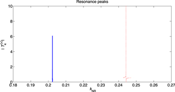
Figure 2. Resonance peaks for Z = 58 and the partial wave  . The two possible spin configurations cause different peaks. The solid line corresponds to the (−) configuration and the dashed line corresponds to the (+) configuration. Each line is truncated on both sides of the corresponding resonant energy;
  for the (−) configuration, and
  for the (+) configuration.
Download figure:
Standard image High-resolution image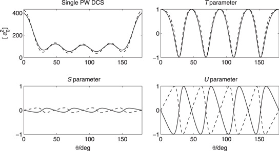
Figure 3. Contribution of the resonant partial wave to the (unpolarized) DCS and the  parameters for
  and Z = 58. A solid line corresponds to the (−) configuration for
  and a dashed line corresponds to the (+) configuration for
  .
.
Download figure:
Standard image High-resolution imageThe  and
and  parameters show an out-of-phase behavior and
  shows an in-phase behavior in figure 3. This is explained at well separated (
 )-resonances by the differing signs of
  and
and  in the spin-flip amplitude
  in (3.2). The oscillations of the
  parameter are small relative to those of the other parameters, indicating that the imaginary part of
  is small.
The oscillations in the parameters  and
and  in figure 3 are wide and attaining the values
  at maxima/minima. This behavior can be analyzed as follows. One concludes from (4.1) and (4.3) that
  attaining a value
  means that
  or
or  vanishes, as then
  and
and  become zero at the peaks of
  . On the other hand, if
  attains a value
  , then (4.3) implies that
  and
and  vanish, which means that
  and that
  is real.
When all partial waves are included in the amplitudes  and
and  at resonance one obtains the thick lines shown in figure 4, the solid lines corresponding to the (−) resonance. The oscillations have become more irregular and it is difficult to clearly see the resonant partial wave signature. The best signature of four minima is seen in the
  parameter. For comparison with the structure obtained off resonance two thin lines are added corresponding to energies higher (dashed) and lower (solid) than both resonance energies.
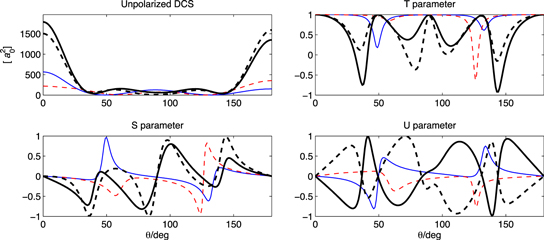
Figure 4. The full (unpolarized) DCS and the  parameters for Z = 58. The thick lines (solid/dashed) correspond to the two resonance energies
  ; see the caption to figure 3. The thin lines correspond to non-resonant energies slightly below (solid) and above (dashed) these resonance energies.
Download figure:
Standard image High-resolution image7.2.
.

The (Z = 54)-potential model has a single isolated resonance for  at
at  [10]. In this case the (−) component resonance is suppressed to a bound state [10]. The remaining energy peak is shown in figure 5 and the resonance signatures are seen in figure 6. In this case the oscillations in
  for the resonant partial wave are also relatively small.
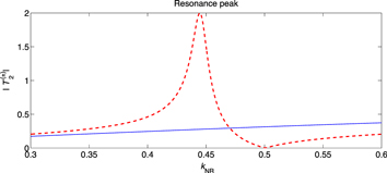
Figure 5. Resonance peak for Z = 54 at  and the partial wave
  . The peak corresponds to the (+) configuration with a dashed line. In this case the peak of the (−) configuration (solid line) does not exist, because this resonance has turned into a bound state [10, 11].
Download figure:
Standard image High-resolution image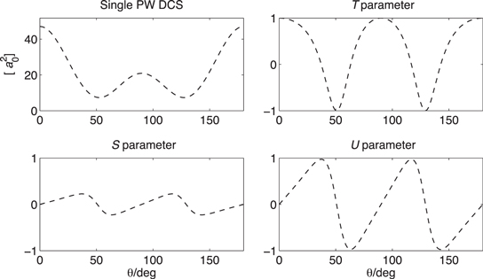
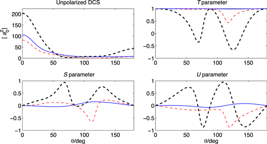
Figure 6. Contribution of the resonant partial wave to the (unpolarized) DCS and the  parameters for
  and Z = 54. Only the (+) resonance at
  exists in this case.
Download figure:
Standard image High-resolution imageThe DCS when all partial waves are included and the  parameters for
  are shown in figure 7. As in figure 4,
  shows a distorted but clear resonance signature in figure 7. The off-resonance patterns (thin lines) for
  being clearly different; the continuous line representing a lower nearby energy is very close to the value
  , and the thin dashed line has only one significant minimum.
Figure 7. The full (unpolarized) PW DCS and the  parameters for
  and Z = 54. The thick dashed lines correspond to the resonance energy of the (+) configuration. The thin lines correspond to energies below (solid) and above (dashed) these resonance energies.
Download figure:
Standard image High-resolution image
8. Conclusions
For the first time this study shows a theoretical analysis of well isolated sharp resonances of polarization scattering using Dirac theory. No experimental measurements related to this theoretical investigation have been found. The many-particle effects associated with electron-atom scattering may not be accurately described by the RTF potential so the results observed here will hopefully stimulate further investigations.
The present model calculations clearly show that the polarization parameter  identifies the partial wave quantum number of the resonance, while the
  and
and  parameters provide less consistent signatures.
For each orbital angular momentum, two energy resonance peaks should appear. The resonance with the (+) configuration appears at a higher, nearby, energy relative to the (−) configuration. Relativistic spin effects for lighter atoms may be small in most electron-atom polarization scattering situations, and resonances of spin pairs may not be well separated. Results of this study may be non-conclusive in such cases.
The energy signature of the resonances analyzed here is seen in the DCS in forward and backward directions as functions of the scattering energy. This is of course also how a resonance energy is detected in a total cross-section. The  and
and  parameters are oscillating angular functions at resonance and are irregular. The single resonant partial-wave contributions however show regular structures that are odd with respect to
  . The best identifier of the resonant partial wave quantum number in this study is the parameter