

Abstract
The characterization of the polarization properties of a quantum state requires the knowledge of the joint probability distribution of the Stokes variables. This amounts to assessing all the moments of these variables, which are aptly encoded in a multipole expansion of the density matrix. The cumulative distribution of these multipoles encapsulates in a handy manner the polarization content of the state. We work out the extremal states for that distribution, finding that SU(2) coherent states are maximal to any order, so they are the most polarized allowed by quantum theory. The converse case of pure states minimizing that distribution, which can be seen as the most quantum ones, is investigated for a diverse range of number of photons. Exploiting the Majorana representation, the problem appears to be closely related to distributing a number of points uniformly over the surface of the Poincaré sphere.
Export citation and abstract BibTeX RIS

Content from this work may be used under the terms of the Creative Commons Attribution 3.0 licence. Any further distribution of this work must maintain attribution to the author(s) and the title of the work, journal citation and DOI.
1. Introduction
In this focus issue, celebrating the International Year of Light, we wish to discuss one of the fundamental properties of a beam of light: its polarization [1]; which can be roughly defined as the figure traced out by the tip of the electric field vector during one optical cycle.
In classical optics, if the field is fully polarized, this figure is an ellipse, which can degenerate into a line or a circle. If the field is completely unpolarized, then the figure is erratic and can only be described in statistical terms. This statistical description must be invariant under any change of the polarization basis: in operational terms, this means that unpolarized light remains invariant under any polarization transformation.
At the quantum level, this picture becomes too simplistic. There are, for example, states that classically are unpolarized, but which do carry a quantum polarization structure. These are called states with 'hidden polarization' [2, 3]. What we will show here is that this is just the first level of a hierarchy of states that at first glance look unpolarized, but are in fact polarized when one looks at higher-order fluctuations.
In order to systematically derive this hierarchy, we shall use the Majorana representation [4], which maps any N-photon state onto N points on the Poincaré sphere. We will subsequently show that the problem we consider, quantum optical states with peculiar polarization properties, is connected to several other seemingly unrelated problems in physics and computational science. We do not yet understand either why or to what extent the problems are related, but intuitively they all boil down to a geometrical problem, namely: what is the optimal configuration if one wishes to place N points on the unit sphere in the 'most symmetric fashion' possible? [5–7].
This paper is organized as follows. In section 2 we review some of the required mathematical concepts. In section 3 we state the problem in more precise terms and in section 4 we present some of the stars of the quantum Universe, i.e. the most unpolarized and therefore the most nonclassical states in a polarization context. Subsequently, in section 5, we discuss several related problems and compare the solutions. In section 6 we speculate about the potential use our stars may have. Finally, in section 7 we make some concluding remarks and explore ideas for the future directions of this research.
2. Basic polarization tools and concepts
We consider a monochromatic, plane field, described by two amplitudes  and
and  representing the annihilation operators of two circularly polarized orthogonal modes, right-handed (+) and left-handed (−), respectively. They obey the bosonic commutation relations
 ![$[{\hat{a}}_{j},{\hat{a}}_{k}^{\dagger }]={\delta }_{{jk}}$](https://content.cld.iop.org/journals/1402-4896/90/10/108008/revision1/ps519237ieqn3.gif) (
( ) and the superscript † stands for the Hermitian conjugate.
The Stokes operators are [8]:

and bear a very simple operational interpretation:  represents the intensity,
  the intensity difference between horizontal and vertical linear polarizations,
  the intensity difference between linear polarizations at
  and
and  and
and  the intensity difference between right- and left-handed circular polarizations. While the last assertion is rather obvious, it is less obvious that
  indeed is the the intensity difference between horizontal (H) and vertical (V) linear polarizations. However, expressing
  and
and  it is straightforward to derive that
  indeed equals
As written in equation (1), they differ by a factor 1/2 from the conventional definition [9], but in this way they satisfy the commutation relations of the  algebra (in units
  throughout)

and cyclic permutations. This noncommutability precludes the simultaneous sharp measurement of the quantities they represent. Among other consequences, this implies that no field state (apart from the vacuum) can have sharp nonfluctuating values of all the operators  simultaneously. This is expressed by the uncertainty relation

where the variances are given by  In other words, the electric field of a quantum state never traces out a definite ellipse. Note that there is a complete formal equivalence between the space of fixed total photon number N with a spin
In addition, we have

and one must therefore address each subspace with a fixed number of photons N separately. This can be emphasized if instead of the two-mode Fock basis  we employ the relabeling

In this way, for each fixed S (i.e., fixed number of photons N), m runs in unit steps from  to S and these states span a (2S+1)-dimensional subspace wherein
  acts in the usual way.
In classical optics the total intensity is a well-defined quantity. In consequence, normalizing the Stokes variables by the intensity determines the unit Poincaré sphere. At the quantum level, as fluctuations in the number of photons are unavoidable, one should talk of a three-dimensional Poincaré space (with axes S1, S2 and S3) that can be envisioned as foliated in a set of nested spheres with radii proportional to the different photon numbers that contribute significantly to the state. But if one limits oneself to a single spin component S and picks one of those nested spheres, we can rightly speak about the unit Poincaré sphere as in the classical world.
The Stokes operators are also the infinitesimal generators of SU(2) polarization transformations; that is

with θ a real parameter, and  a normalized, three-dimensional, real vector. These are all linear energy-preserving transformations of the field amplitudes, embracing every optical operation of phase plates and rotators. It can be seen that the action of
  on
on  is a rotation of angle θ around an axis

Observe that given the rotation  with
with  both
both  and
and  lead to
The relation (4) implies that the polarization properties of any quantum state can be analyzed by splitting its density matrix into a direct sum of finite-dimensional components

where  is the density matrix in the subspace of spin S. This
  has been termed the polarization sector [10] or the polarization density matrix [11].
Instead of using the states  in the following we will expand
  as
as

The irreducible tensor operators  are [12, 13]

with  being the Clebsch–Gordan coefficients that couple a spin S and a spin K (
 ) to a total spin S. The tensors
  constitute an orthonormal basis and have desirable properties under SU(2) transformations. An important property is that
  can be written down in terms of the Kth powers of the Stokes operators (1). In particular, if for a given pair of S and M all coefficients
  vanish for
  irrespective of q, then the moment
  (with
(with  ) will be isotropic and independent of
  Clearly, this then also holds for all moments
  where
where 
The expansion coefficients  are known as state multipoles. Hence,
  is just the square of the overlap of the state with the Kth multipole pattern in the Sth subspace. For most states only a limited number of multipoles play a substantive role and the rest of them have quite a small contribution. Therefore, it seems that a convenient way to quantify the polarization information is to look at the cumulative distribution

which conveys all the information up to order M. Note that the monopole term  is excluded, as it is just a constant term. As with any cumulative distribution,
  is a monotone, nondecreasing function of the multipole order. Using (9) and the fact that the tensor operators are orhonormal we see that

so for a state with a fixed S,  is equal to the state's purity [14–16] (minus the monopole contribution
  ).
).
We shall be mainly interested in dealing with pure states belonging to a specific excitation manifold S. Accordingly, if we expand the state as  with coefficients
  we can then recast (11) as

3. Classical versus quantum polarization states
Given a fixed spin S, the classical configuration space is the unit sphere associated with the SU(2) symmetry. The SU(2) coherent states in this case can be identified with a point on the sphere obtained by a rotation of the North pole  [17, 18]. There is a consensus that they are the most classical states, as they have all their polarization aligned in one direction. Besides, they have nice extremal properties, such as minimal total variance of
  [19] or minimal Wehrl entropy [20].
In our context, it is remarkable that they have maximal aggregated multipole strength  for any order M [15, 21]. It is irresistible to ask which states attain the minimum of this magnitude, as they can be considered in a sense as 'the opposite' of SU(2) coherent states and so the most nonclassical ones. This appears to be closely related with a proposal that has met with considerable interest: anti-coherent states, defined as the states that have a vanishing Stokes vector as well as isotropic Stokes variances [22].
A useful tool in this context is the Majorana representation of a pure N-photon state [4], which is based on the fact that any such state  (where the reader is reminded that
  ) can be written as [23]

where  is a normalization factor, and the angles
  and
and  satisfy the natural constraints
  and
and  Thus, each factor in (14) can be pictured as a point on the unit Poincaré sphere. Since the operators
  and
and  create an excitation in right- and left-hand circularly polarized modes, respectively, each of the factors in (14) can also naively be thought of as creating an 'excitation component' with a polarization state corresponding to its position on the sphere. The resulting configuration of points is called the Majorana constellation associated to the state
  An illustration of these ideas is schematized in figure 1.

Figure 1. The star denotes the Majorana constellation of the state 

 The four red dots give the constellation for the S = 2 N00N state in equation (17).
Download figure:
Standard image High-resolution imageWe associate the North (South) pole with right- (left-) handed circular polarization and thus the equator represents different linear polarization excitations. For example, the N-photon SU(2) coherent state  is represented by N points at the North pole of the sphere so that all 'excitation components' have identical (right-handed) circular polarization.
An SU(2) rotation simply corresponds to a solid rotation of the Majorana constellation. Thus, states with the same constellation, irrespective of its relative orientation, have the same polarization invariants. Intuitively, one would guess that states with polarization as isotropic as possible would have a constellation as symmetric as possible.
To place this guess in a more rigorous mathematical frame, one can go beyond the variance, and look for the states that have isotropic polarization properties for all the moments  [22, 24, 25]. For a given S, one cannot find pure states that have isotropic moments up to order
  only completely mixed states have this property [26, 27]. Thus, for each S there exists a set of pure states that are unpolarized up to a maximal degree M. These Mth-order unpolarized states are the stars of the quantum Universe. Below we shall sometimes be a bit imprecise and speak about a constellation as a state, which is evident from (14).
4. Stars of the quantum Universe
To find the Mth-order unpolarized states for a given S, we start from a set of  amplitudes
  where
where  are real numbers, as in equation (13). Since the orientation of the constellation is irrelevant we can reduce the number of variables by fixing one of the points to be at, say, the North pole and another to lie in the the S2–S3 plane. We subsequently try to get
  for the highest possible M, which amounts to setting the state multipoles
  to zero. This leads to a system of polynomial equations of degree two for am and bm, which we solve using Gröbner bases [28] implemented in the computer algebra system MAGMA [29, 30]. In this way, we get exact algebraic expressions, and we can detect when no feasible solution exists.
Our results can be summarized as follows. For small values,  the parameter space is simply too small even to allow for states with isotropic variance. For S = 1 and
  one can find states with vanishing Stokes vector, but all such pure states have non-isotropic variance [21] and so they present hidden polarization [2]. The S = 2 excitation manifold is the first allowing a second-order unpolarized state. However, the space is still so small that the solution is unique. For
  no second-order unpolarized state exists. For larger numbers,
  there exist several different constellations that all are unpolarized to the same order M, but that are not simply connected by a unitary polarization transformation. We have not yet found a way of assuring that we find all constellations for a given S, nor have we found a general way of asserting with certainty that for a given S we have found the constellations that maximize M. This is related to the fact that with growing S, the number of different maximally unpolarized constellations grows and it becomes more difficult to show that the corresponding system of polynomial equations has no solution over the real numbers. The same kind of difficulties appear in several related problems such as spherical t-designs, the Thomson problem, and the Queens of quantumness that will be discussed in the next section. However, after spending considerable time on computer searches, we are fairly confident that the constellations we present are indeed optimal.
Let us now look at some of the stars of the quantum Universe. A list of star states having S = 1 to 10 can be found in the Supplementary material file, available at stacks.iop.org/ps/90/108008/mmedia. Note that for most values of S, except for the smallest, there exist many inequivalent star states. As exemplified in figure 3, below, in general they have different cumulative multipole distributions  For more complete information and lists over inequivalent star states for different values of S, the reader is referred to [31].
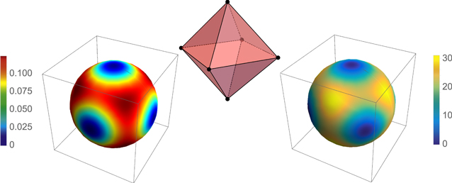
Figure 2. Density plots of the SU(2) Q-function (left) and the first non-isotropic moments  (right) for the maximally unpolarized state
  in the excitation manifold S = 3. In both cases, we have used a pseudo-color map with the indicated scales. On top, we have given the Majorana constellation of the state, which is a regular octahedron inscribed in the Poincaré sphere. Note that the vertices coincide with the zeros of the Q function, but not with the zeros of
Download figure:
Standard image High-resolution image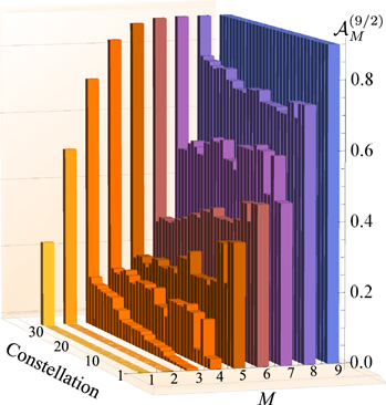
Figure 3. The multipole cumulative distribution  as a function of the multipole order M for all the 31 maximally unpolarized constellations we have found for
  . The last constellation, number 32, corresponds to an SU(2) coherent state, taken as a reference.
Download figure:
Standard image High-resolution image
 The least excited second-order unpolarized state is the four-photon state. Its Majorana constellation is a regular tetrahedron and this configuration is unique. The corresponding state is
  (and, of course, all states on its SU(2) orbit).
 Five is a number that does not allow a high degree of spherical symmetry. Based on an elementary counting, it was conjectured in [22] that five-photon anti-coherent states would exist. However, some time later it was proven that one can only find first-order, but no second-order unpolarized states [32]. The constellation consists of the vertices of an equilateral triangle inscribed in the equator, plus the two poles.
 Now another Platonic solid appears, the regular octahedron. The corresponding state, which is unique up to SU(2) transformations, is
  This is the least excited state that is third-order unpolarized. Since
  for odd M, all odd order Stokes operator moments must vanish for them to be isotropic (irrespective of S). This state, like all states that have isotropic variance, has the maximum sum of Stokes operator variances. Since for any unpolarized state
  the relation (3) imposes the bound

All second-order unpolarized states saturate the upper bound in the inequality above [22]. Thus, all maximally unpolarized states with  fulfill
  in any direction
  on the Poincaré sphere. In figure 2 we plot the Majorana constellation, the Q-function, and the first non-isotropic moments (M = 4) as a function of the direction on the Poincaré sphere for this state.
 In this space there are at least 31 different constellations with six different abstract symmetry groups that are second-order unpolarized, but we conjecture that no third-order unpolarized constellations exist. The constellations differ in how the aggregated multipole strength
  increases with M. We have found 20 different such functions and they are plotted in figure 3. The constellation with the smallest third-order multipole strength has
  and the one with the largest has
  The former case is generated by three equilateral triangles: one inscribed in the equator and the other in two rings symmetrically placed above and below the equator. The middle triangle is rotated 60° around the polar axis with respect to the other two. The corresponding state is
The  case is rather typical for
  several different constellations unpolarized to the same (maximal) order exist. Different constellations may have the same or different accumulated multipole strength
  as a function of M.
For some values of S, such as 4, 6, 8, 12 and 20, one can guess a maximally unpolarized constellation, in each case corresponding to the vertices of a Platonic solid. For other numbers such as  it is not easy to guess an optimal, 'exact' constellation, but solving the system of polynomial equations, as described at the beginning of this section, yields exact algebraic expressions for the coefficients
  from which one can easily compute the points of the Majorana constellation with arbitrary numerical precision.
5. Other spherical configuration problems
The problem of distributing N points on a sphere in the 'most symmetric' fashion has a long history and many different solutions depending on the cost function one tries to optimize [5, 6]. Here, we shall only discuss a few of the formulations: spherical t-designs [33–35], the Thomson problem [36–39] and the Queens of quantumness [40]. We leave out the connections to other intriguing problems, such as as maximally entangled symmetric states [41, 42], k-maximally mixed states [43], and states with maximal Wehrl–Lieb entropy [44].
Spherical t-designs are configurations of N points on a sphere such that the average value of any polynomial of degree at most t has the same average over the N points as over the sphere. Thus, the N points can be seen to give a representative average value of any polynomial of degree t or lower. Such designs can be found for (hyper)spheres of higher dimensions, but to connect to the stars we will only consider t-designs on the three-dimensional sphere. It has been conjectured that a state is t-order unpolarized if and only if its Majorana constellation is a spherical t-design [24]. However, although the statement is true for some t-designs, such as those represented by the Platonic solids, the conjecture is not true in general [25].
It is clear that there must be some connection between the number of points that are at one's disposal and the maximal degree t for which an N point configuration allows for a spherical t-design. The configurations that maximize t for a given N are called optimal designs, and in the following t will denote the degree of an optimal N-point design. No analytical expression is known between N and t: it is known that for a t-design in three-dimensional space, the number of points N is at least proportional to t2, whereas for some orders t only constructions are known for which N scales proportionally to t3. As a function of N, the order t is non-monotonic. The current state of knowledge is summarized for  in [35]. In table 1 we list some maximally unpolarized constellations and their corresponding optimal t-designs.
Table 1. Some designs on a sphere and their respective degrees of unpolarization M. 'same' and 'similar' always refer to the closest description column to the left. Explicit expressions for the stars of the quantum Universe for several values of S can be found in [31].
| S | Quantum stars | M | t-design | t | M | Thomson | M | Queens | M |
|---|---|---|---|---|---|---|---|---|---|
| 1 | Radial line | 1 | same | 1 | 1 | same | 1 | same | 1 |
| 3/2 | Equatorial triangle | 1 | same | 1 | 1 | same | 1 | same | 1 |
| 2 | Tetrahedron | 2 | same | 2 | 2 | same | 2 | same | 2 |
| 5/2 | Equatorial triangle + poles | 1 | same | 1 | 1 | same | 1 | same | 1 |
| 3 | Octahedron | 3 | same | 3 | 3 | same | 3 | same | 3 |
| 7/2 | Two triangles + pole | 2 | similar | 2 | 0 | equatorial pentagon + poles | 1 | same | 1 |
| 4 | Cube | 3 | same | 3 | 3 | square antiprism | 1 | see [40] | 1 |
| 9/2 | Three triangles | 2 | similar | 2 | 1 | three staggered triangles | 1 | similar | 1 |
| 5 | Pentagonal prism | 3 | similar | 3 | 1 | two staggered squares + poles | 1 | same | 1 |
| 6 | Icosahedron | 5 | same | 5 | 5 | same | 5 | NA | — |
| 7 | Four triangles + poles | 4 | same | 4 | 1 | two hexagonal rings + poles | 1 | NA | — |
| 10 | Dodecahedron | 5 | same | 5 | 3 | see [38] | ? | NA | — |
Several interesting conclusions can be drawn from table 1. First, the maximum M and t coincide. In fact, this has been the case for any excitation manifold we have studied, and these include all S up to 24, with some omissions. We therefore conjecture that if an optimal spherical design of order t exists for some N, then one can find an Mth-order unpolarized N-photon state with M = t.
The next thing one can note is that an optimal t-design does not necessarily give a tth-order unpolarized state. Quite often the configurations are similar, e.g. regular polygons with their surface normals along the polar axis, but displaced from each other along the axis by certain distances. However, these distances need often be fine-tuned for an optimal t-design to become a star. The Platonic solids are exceptions to this observation. That the optimal configurations for t-designs and maximally unpolarized states do not coincide underscores the 'mystery' that the optimal t and maximal M always seem to be equal for any N (or equivalently, for any S).
Another similarity between optimal spherical t-designs and the stars of the quantum Universe is that the configurations typically are not unique, aside from the smallest dimensions.
The Thomson problem consists of arranging N identical point charges on the surface of a sphere so that the electrostatic potential energy of the configuration is minimized. For N = 2 the solution is easily visualized: the repelling force tends to place the charges on antipodal points of the sphere, thereby maximizing the distance between them. The problem can be generalized to potential energies of the form  where r is the Euclidian distance between the charges. The choice d = 1 is the Thomson problem, corresponding to the usual Coulomb potential and it is the one we will focus on in this work. The case
  is called Tammes problem [45].
In table 1 we have listed the optimal Thomson configurations and the degree of unpolarization of the corresponding state. We see that for small S, up to 3, the configurations are identical to the optimal spherical t-design and to the stars. For larger S, they differ in general and the degree of unpolarization of the 'Thomson' states is lower than the maximum. Different from the two previous cases, the solution of the Thomson problem appears to be unique for every S [46].
The Queens of quantumness are the states that maximize the Hilbert–Schmidt distance to the closest point of the convex hull of the mixed SU(2) coherent states [40]. This convex hull defines the subspace of classical states. Therefore, the states maximizing the distance to the nearest point on this hull can be thought of as having maximally quantum characteristics. In [40] it is claimed that the Queens can be seen as the least classical (or most quantum) of all states given this metric. Although we have used another figure of merit, our approach and that in [40] share the view that the states 'most different' from SU(2) coherent states are the most nonclassical.
It is not surprising that the Queens turn out to be anti-coherent (second-order unpolarized) when possible, since they should be as 'far away' from the SU(2) coherent state as possible. In table 1 we have also listed the configurations and the degree of unpolarization for these states. These configurations also seems to be unique, contrary to the maximally unpolarized states and the optimal spherical t-designs. We also see that the Queens are not maximally unpolarized except when 
6. What are the applications?
In deriving the maximally unpolarized states we have simply been driven by the quest for the most nonclassical states from a polarization perspective. Yet, the remarkable properties of such states make them potential candidates to outperform classical states in certain tasks.
The salient feature of the stars is their ability to signal small, but arbitrary SU(2) transformations with optimal resolution. This has already been anticipated in [32], where the authors specifically found that for photon numbers 4, 6, 8, 12 and 20, the states corresponding to regular polyhedra Majorana constellations best signal misalignments between two Cartesian reference frames. To understand this, it is instructive to look at related states, namely the N00N states

Such N00N states are known to have the highest sensitivity for a fixed excitation S to small rotations about the  -axis [47]. Their Majorana constellation consists of
  equidistantly placed points around the Poincaré sphere equator. For example, the state
  can be written

That is, the four Majorana points are 

 and
and  as sketched in figure 1. The angle between any two adjacent points is
  while for a general N00N state of the form (16), this angle is
A rotation around the  -axis is described by the unitary operator
  We have that for
  the states
  and
and  are orthogonal, whereas for
  they are parallel, where q is an integer. Thus, it should not come as a surprise that N00N states are optimal for detecting small rotations around the
  -axis, in the interval
  However, as soon as the rotation exceeds the upper bound in this inequality, one will have difficulties in resolving the rotation angle, as two or more rotation angles will result in the very same rotated state. If the rotation axis lies in the equatorial plane, then a rotation of π is needed to get a parallel state, irrespective of S. This happens only if the axis intersects one of the Majorana points when S is a half integer, or if the axis intersects either a point or is the intersector between two points if S is an integer. Thus, the rotation resolution is highly directional for a N00N state.
The situation is to some extent similar and to some extent different for the stars of the quantum Universe. It may not be obvious from their appearance that they have high sensitivity to small rotations around an arbitrary axis. To substantiate this claim, recall that the action τ needed to make a state  evolve so that
  where
where  is a small, positive, real number, and
  is Hermitian, is inversely proportional to the state's variance
  [48]. The relation connecting the evolution speed
  and the variance is sometimes called the 'quantum speed limit' [49, 50]. A N00N state in the
  basis has maximal variance
  for a fixed S and thus is the state with maximal sensitivity for a rotation around the
  axis. However, the state's
  and
and  variances are only
  and thus the state is rather insensitive for rotations around those axes (or to any rotation axis in the
  –
– plane). However, all the star states have isotropic variances equal to
  that is, close to the maximum. The proof of this statement is as follows:
The second expression from the left follows from the fact that the star states have vanishing mean first order moments  Since their variance per definition is isotropic, we also have that
  Having a large, and isotropic variance of the Stokes operator, the quantum speed limit theorem thus asserts that these states are rather sensitive to rotations around any axis
Another way of explaning the star states' sensitivity to a rotation around an arbitrary axis is to observe that, since these states have 'maximal' spherical symmetry, they become parallel, or almost parallel, for relatively small rotations around several axes. For example, for the Platonic solids, rotations around all the facets normal axes map the Majorana constellation onto itself (resulting in a parallel state) for rotations of  (tetrahedron, octahedron and icosahedron),
  (cube), or
  (dodecahedron). For other constellations and other rotation axes the Majorana constellation will only become approximately identical, but the problem with resolution of large rotations will predominantly remain. However, having a high degree of spherical symmetry, the maximally unpolarized states will resolve rotations around any axis approximately equally well. To quantify this statement one could use the Fisher information and the Cramér–Rao bound to assess the uncertainty in estimating the rotation direction and the rotation angle [49, 50]. Such an investigation lies outside the scope for this paper, but work along this direction is in progress.
To conclude, we stress that there is also some structural similarity between the stars of the quantum Universe and quantum error correcting codes. In both cases, low-order terms in the expansion of the density matrices vanish. The putative application of the stars for error correction constitutes an important goal for our future research.
7. Conclusions
We have derived a class of pure states that lack polarization properties to the lowest orders. They can be seen as generalizations of states with hidden polarization and the anti-coherent states. We call them stars of the quantum Universe and they are Mth-order unpolarized: the moments  are isotropic for
  We find, so far to our surprise, that although their respective Majorana constellations do not necessarily coincide, we always find that for a pure N-photon state, the highest possible degree of unpolarization is M = t, where t is the maximal degree for an N-point spherical t-design. Our conjecture is that this is indeed true for any N.
We have also discussed the possible connections between the Majorana constellations for the stars and some other problems involving symmetry of points on a sphere, namely the Thomson problem and the Queens of quantumness. The conclusion is that although the problems are related, the fact that the solutions coincide for small dimensions is surely due to the limited degrees of freedom low-dimensional systems offer. When the dimension becomes larger, say involving more than ten points, the solutions are no longer identical except perhaps for when 'exact' symmetry is possible, as is the case for the Platonic solid constellations.
The maximally unpolarized states are an academic curiosity in that they can be said to be the most nonclassical polarization states. In a more practical setting, they seem to be the optimal states for detecting small SU(2) rotations around an arbitrary unknown axis. However, there are still many things to explore: for example, what is the significance of the strength of the first nonzero multipole of a maximally unpolarized state? The cumulative distribution  may increase in different ways as seen in figure 3, but since
  for any pure state, a slower growth for small M must be compensated by a faster growth for larger M. What difference do different constellations make on the fundamental and on the application level?
It is also still unclear why there seems to be such a strong connection between spherical t-designs and maximally unpolarized states. In particular, this connection seems unjustified, as the optimal Majorana constellations do not coincide.
In summary, one can use the example of maximally unpolarized states to marvel about the connections between different branches of science, and on how some seemingly simple problems—distributing points in the most symmetric manner on a sphere—can illuminate such complicated optimization problems that we have just described. The science of light is fantastic!
Acknowledgments
The authors acknowledge interesting discussions with Daniel Braun, Olivia di Matteo and Juan J Monzón. Financial support was obtained from the Swedish Research Council (VR) through its support of Linnaeus Center of Excellence ADOPT and by Grant No. 621-2011-4575. We also thank the European Union FP7 (Grant Q-ESSENCE), the Spanish MINECO (Grant FIS2011-26786) and the Program UCM-BSCH (Grant GR3/14). GB thanks the MPL for hosting him and the Wenner-Gren Foundation for economic support during the autumn of 2014.