

Abstract
This paper investigates the issue of adaptive finite-time control for hyperchaotic Lorenz–Stenflo systems with parameter uncertainties. Based on finite-time Lyapunov theory, a class of non-smooth adaptive finite time controllers is given to guarantee the adaptive finite-time stability and make the states of the systems converge to the origins within a finite-time. Finally, illustrative examples are presented to verify the effectiveness of the proposed adaptive finite-time controller.
Export citation and abstract BibTeX RIS
1. Introduction
Since American meteorologist Edward Lorenz discussed chaotic phenomena in 1963 [1], chaotic behavior has been widely studied in many areas, such as engineering science, medical science, biological engineering, and secure communication. In many practical systems, as an undesirable phenomenon, chaos may lead to oscillation or irregular movement and even collapse of the systems. Therefore, chaos control aimed at eliminating the undesired chaotic behavior has become an important issue in the field of nonlinear control.
Since the celebrated Ott–Grebogi–Yorke control method was given in [2], chaos control has attracted much attention [22–23, 31]. Many researchers have adopted adaptive control methods to suppress chaos in chaotic systems with unknown parameters [3–8]. Most of them considered asymptotic stability of the system, while finite-time stability may make more sense in some practical situations. As an effective method for the control of nonlinear systems, finite-time control can make the system states converge to an equilibrium point in a finite time. Studies have shown that finite-time control can make systems have better robustness or disturbance rejection properties [9–11, 13, 14, 28]. To achieve faster convergence speed and better local robustness in control systems, the finite-time control method is effective.
In recent years, many researchers have done a lot of work on modeling and analysis of finite-time control of chaos [15–20]. Reference [20] investigated finite-time chaos synchronization between two different chaotic systems with fully unknown parameters. If we suppose that the state variables of the master system are all equal to zero, then the problem becomes chaos control, which is similar to our problem. However, in paper [20], the upper bounds of the unknown parameters are assumed to be available, and it may be hard to get the upper bounds of some parameters in certain practical situations. So, an adaptive finite-time control method without known upper bounds of parameters is proposed to eliminate chaos in the permanent magnet synchronous motor (PMSM) system with unknown parameters in [12]. However, in reference [12] the model equation is 3rd-order systems with two uncertain parameters. In this paper, an adaptive finite-time control method without known upper bounds of parameters is proposed to eliminate chaos for hyperchaotic Lorenz–Stenflo systems (4th-order systems with four uncertain parameters) [21].
The organization of the paper is as follows. The preliminary results are given in section 2, which will be used in the sequel. In section 3, an adaptive finite-time control law is proposed for a class of nonlinear systems with uncertain parameters. In sections 4 and 5, some simulation results are provided to show the effectiveness of the proposed method and the robustness of the designed controller. Finally, some concluding remarks are discussed in section 6.
2. Preliminaries
Definition 1. [25] Consider the nonlinear dynamical system

The equilibrium x = 0 of the system is uniformly finite-time stable if there exists an open neighborhood  of the origin and a function
  , called the settling-time function, such that the following statements hold:
- 1.Finite-time convergence: for every
 and , the solution is defined on , for all , and
- 2.Uniform Lyapunov stability: for every, there exists such that , and for every , for all and every .


Finally, the equilibrium x = 0 of the system (1) is globally uniformly finite-time stable if it is uniformly finite time stable with 
Lemma 1. [25] Consider the nonlinear dynamical system (1). If there exists a continuous differentiable function  , class
  functions
  and
and  , a function
  such that
  for almost all
  , a real number
  , and an open neighborhood
  of the origin such that
hold, then the equilibrium x = 0 of the system (1) is uniformly finite-time stable with settling-time function  satisfying
 ![$T({{t}_{0}},{{x}_{0}})\leqslant {{K}^{-1}}[\frac{V{{({{t}_{0}},{{x}_{0}})}^{1-\lambda }}}{1-\lambda }]$](https://content.cld.iop.org/journals/1402-4896/90/2/025204/revision1/ps505227ieqn28.gif) , where
, where  . If
. If  , then the equilibrium x = 0 of the system (1) is globally uniformly finite-time stable.
Definition 2. [26] Consider the following nonlinear system

where f and G are smooth with  and
and  , and θ is an uncertain parameter vector. The problem of global adaptive finite-time stabilization is to find a dynamic controller law

such that the trajectory  of system (3) is globally bounded, and, moreover, for any initial condition
  , x(t) converges to 0 in finite time. In other words, for any initial condition
  , there exists
  such that
  for any
  .
.
Lemma 2. [27] If the solution  of system (1), for any initial condition
  at t = 0, converges to 0 asymptotically when
  , and there is a neighborhood U of x = 0 such that
  of system (1), for any initial condition
  , converges to 0 in finite time, then
  of system (1), for any initial condition
  , converges to 0 in finite time.
This lemma shows that global asymptotic convergence and local finite-time convergence imply global finite-time convergence. This is based on the fact that global asymptotic convergence implies that any solution will enter the given neighborhood U of x = 0 in finite time.
Lemma 3. (Jensenʼs Inequality [29])

where  , and
, and  ,
,  .
.
Lemma 4. (Barbalatʼs lemma [23, 30])
If the differentiable function f(t) has a finite limit as  and if
  is uniformly continuous, then
  as
as  .
.
3. Adaptive finite-time control
We consider the hyperchaotic Lorenz–Stenflo systems as follows:
where ![$x={{[{{x}_{1}},{{x}_{2}},{{x}_{3}},{{x}_{4}}]}^{T}}\in {{R}^{4}}$](https://content.cld.iop.org/journals/1402-4896/90/2/025204/revision1/ps505227ieqn53.gif) is the state vector,
is the state vector, ![$u={{[{{u}_{1}},{{u}_{2}},{{u}_{3}},{{u}_{4}}]}^{T}}\in {{R}^{4}}$](https://content.cld.iop.org/journals/1402-4896/90/2/025204/revision1/ps505227ieqn54.gif) is the control input,
is the control input,  is a nonlinear vector field, and
  is a constant system matrix with unknown elements
  and d. It is obvious that x = 0 is an equilibrium point of system (6).
Theorem 1. The equilibrium point  is adaptively finite-time stabilizable if the dynamic controller is selected as follows:
where  .
.  and
and  are time-varying functions to estimate γ and σ, respectively.

where  ,
,  ,
,  , and
, and  . Take
  , then
Hence, the dynamic controller (7) guarantees that the solution  is globally bounded. V(t) is monotonically decreasing with respect to time t because
  . Moreover,
  is lower bounded; hence
  exists and is finite. It is not difficult for us to get that
  is globally bounded because the right-hand side of the system (6) with the dynamical controller (7) is globally bounded. Then
  is uniformly continuous with respect to time t. According to Barbalatʼs lemma, we can get that
  . Based on the negative definiteness of
  with respect to x, we can get that
  .
.
Let  and
and  . Clearly, from (8),
  ; hence
  . We can get that
  . If let
when  we can get
If we define  and
and  , based on Jensenʼs Inequality, when
  we can have
It is not difficult for us to get that when  , we have
On the other hand, if the initial condition  =
=  , it is not hard to see that
  because of
  ; therefore, for any initial condition
  ,
,  , which implies that the origin of the system (6) is locally uniformly finite-time stable, according to lemma 1. Therefore, based on lemma 2, it is obvious that for the closed-loop system (6), x=0 is globally adaptively finite-time stabilizable. □
4. Numerical simulations
To show the effectiveness of adaptive finite-time control law (7) in hyperchaotic Lorenz–Stenflo systems with fully unknown parameters, the simulation results are provided in figures 1 and 2. The system is simulated for 10 s in a chaotic mode, and then the controller is switched on. The parameter values of the hyperchaotic Lorenz–Stenflo systems are assumed as:  , and
, and  ; the initial conditions are:
  ,
,  ,
,  ,
,  ,
,  . We choose the parameters in theorem 1 as:
  .
.

Figure 1. The state variables of the hyperchaotic Lorenz–Stenflo systems.
Download figure:
Standard image High-resolution image
Figure 2. The time variations of the estimated parameters.
Download figure:
Standard image High-resolution imageFrom figures 1 and 2, we can see that it only takes a very short time to eliminate the chaos in the hyperchaotic Lorenz–Stenflo systems and adaptively finite-time stabilize the system at the equilibrium point  .
.
The robustness of a closed-loop system is also an important issue in control theory. In order to analyze the robustness of the presented control method, the following disturbed models are considered:
where

We use the same adaptive finite-time control law to control the disturbed system (8) with the initial conditions  ,
,  ,
,  ,
,  and
and  and get figures 3 and 4.
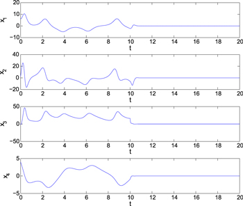
Figure 3. The state variables of the disturbed hyperchaotic Lorenz–Stenflo systems.
Download figure:
Standard image High-resolution image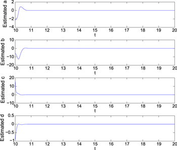
Figure 4. The time variations of the estimated parameters of the disturbed systems.
Download figure:
Standard image High-resolution image
5. Conclusions
In conclusion, the adaptive finite-time stabilization of the the hyperchaotic Lorenz–Stenflo systems is investigated in this paper. Based on finite-time stability theory and the adaptive control method, an adaptive finite-time control law is proposed. The simulation results show the effectiveness of the proposed method and the robustness of the designed controller.