

Abstract
The bipolar motor is a compass in an oscillating magnetic field. It has been intensively studied as a system exhibiting chaos in the years 1980–1990. It was a trendy system, easy to build and to model. However, several regimes reachable by the compass has been left unspoken. The compass can rotate, oscillate or stop depending on internal or exciting parameters. It can also develop parametric instabilities under specific conditions. The goal of this paper is to explain and predict the transition between those regimes and their organization in the parameter space made up of the magnetic field amplitude B and its frequency ωB. This work is tackling the range of non-chaotic behavior of the compass and it will not overlap the previous studies of the deterministic chaos regimes. It will compare experimental, numerical and theoretical results and demonstrate good agreement between them.
Export citation and abstract BibTeX RIS
1. Introduction
A bipolar motor is a simple system which exhibit a great number of nonlinear phenomena. It is composed of a compass in an oscillating magnetic field. It is an experiment that can be easily presented to students for Chaos route demonstration and it was its purpose in the years 1980–1990. Several authors developed experiments [1–5], models [6] and simulations [7, 8] of the compass deterministic chaotic behavior. However, despite deep studies of the chaos characteristic, a part of possible regimes has been put aside by the community: the rotation and the oscillation of the compass. The goal of this study is to set measurements, analytical calculations and simulations of those bipolar motor periodic regimes. The framework of this paper is the parameter space made up of the magnetic field amplitude B and its frequency ωB. We will explicit how periodic regimes surround the chaotic regions and also detail the parametric instabilities thresholds.
The paper is organized as follow: section 2 describes the bipolar motor. Section 3 provides the results on the rotation regime. Section 4 is about the space parameter region that contains the chaotic motion. Section 5 details the parametric instability of the system. Section 7 presents dynamics limitations of the rotation regime.
2. Physical setup
The experimental device is illustrated in the scheme figure 1. The large coil (30 cm diameter) produces the magnetic field that drives the compass dynamics. The compass (3 cm diameter) is fixed inside the coil with two bearing balls. Two hall effect sensors are set around the compass, one along the coil axis and the other perpendicular to it. The combination of the two signals allows a direct measurement of the compass angle θ(t) at a frequency rate of 1 kHz. The compass and the sensors are described in details in [9]. The magnetic field is controlled by a program that sets its amplitude B and its frequency ωB. Modifications of B and ωB can be triggered at a chosen compass angle θi and rotation speed ωi, which will be the initial condition of the compass.

Figure 1. Scheme of the device. Orange: the coil that produces the magnetic field. Blue: the bearing balls that fix the magnet. Green: the permanent magnet. Black: the referential and the sensors.
Download figure:
Standard image High-resolution imageThe compass dynamics is governed by the following equation:

θ is the angle between the magnetic field direction and the compass magnetic moment M = 0.77 A m2. J is the compass inertial moment equal to 8.35 × 10⁻⁷ kg m2. F is the fluid friction coefficient equal to 0.10 × 10⁻⁵ kg m2 s−1. Methods used to determine the system parameters are explained in appendix A. The magnetic field has a sinusoidal form:  . Depending on the frequency, the magnetic field can reach up to 10 mT. There are several possible regimes presented in figure 2. The compass can oscillate between the two directions of the coil axis at the magnetic field frequency (a). It can have a chaotic behavior (b). It can rotate at the magnetic field frequency (c). Finally, the compass can stop its rotation and align along one direction of the coil axis (d).
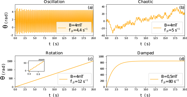
Figure 2. Experimental evolutions θ(t): (a) Oscillation (b) Chaotic (c) Rotation (d) Damped.
Download figure:
Standard image High-resolution imageWe aim at sorting the conditions of observation of those regimes in the parameter space (B, fB). We start by considering the rotation regime.
3. Rotation of the compass
When the compass is rotating with the magnetic field, the model equation (1) can be simplified using the periodicity of the rotation. The average speed of the compass is ωB and the compass average acceleration is null. The Lorentz force has to compensate the friction of the fluid: this is only possible if the compass has an average phase shift delay with the magnetic field, quoted as ϕ. The solution of the rotating regime has the form: θ = ωBt + ϕ. Casting this solution in equation (1) and making the average of this equation over one turn, one obtain:

Assuming a positive rotation, ϕ is limited by two values: −π or −π/2. In the limit of null friction, ϕ = π/2 and the Lorentz force does not need to sustain the rotation. The motion can be described by quarters of TB, the period of the magnetic field oscillation. During the first quarter of TB, the compass goes from −π/2 to 0. The magnetic field increases from 0 to B and accelerates the compass. During the second quarter of TB, the magnetic field reduces from B to zero and the compass decelerates. The phase shift of −π/2 produces a null Lorentz force in average over half a turn. For a large fluid friction,  . The Lorentz force is always accelerating the compass but all the energy provided by the magnetic field is consumed into the fluid friction. If the frequency fB increases or the magnetic field amplitude decreases, the energetic balance in half a period may be negative and the rotation condition is lost. The rotation is possible if
  which sets our first limitation in the parameter space
 ![$[B,{f}_{B}]$](https://content.cld.iop.org/journals/1402-4896/94/1/015002/revision2/psaaecf3ieqn4.gif) . The rotation is sustained if
. The rotation is sustained if

The phase shift equation (2) is compared to measurements in figure 3. The two limits of ϕ are observed including the rotation lost at B = 0.2 mT when ϕ ≃ −π. The rotation condition equation (3) is also measured experimentally by slowly reducing the amplitude of the magnetic field during the rotation regime for several fixed frequencies. Figure 4 shows that those measurements and the analytical limit are in a very good agreement. The interpretation of the phase shift ϕ suggests that there is an oscillation of θ(t) around ϕ during the rotation, see the insert in figure 2(c). This can be casted in the solution of the equation as a function δ(t): θ = ωBt + ϕ + δ(t). We obtain by gathering this form of the solution and the equilibrium equation (2) into the model equation (1):
In the case of small oscillations (δ(t) < 1), the nonlinear second right hand side term can be neglected compared to the first which is the source of the oscillations. The solution for δ(t) must have a null average to satisfy the rotation constraint. Then the solution is:
with  , the eigen frequency of the compass. As expected, the frequency of oscillations is twice the rotation speed: one per half-turn. For a 10 Hz rotation, we have 2ωB ≫ F/J and we can deduce from equation (5) the amplitude of the second harmonic in ωB:

This value is obtained from experimental and numerical data with a Fourier analysis of δ(t) for different B at 10 Hz. There is a good agreement for δ2 between experimental, numerical and analytical results, showed on figure 5. For the larger magnetic field presented on figure 5, δ2 is about 0.17 which still satisfies our hypothesis. However the numerical results show a different behavior for B > 6.2 mT. This behaviour will be described in sections 4 and 5.
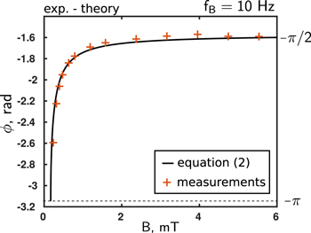
Figure 3. Phase shift between the compass and the magnetic field versus the magnetic field amplitude at the exciting frequency. Crosses for measurements. Black line for analytical solution equation (2). The phase shift measurement is an average of ϕ over several turns of the compass.
Download figure:
Standard image High-resolution image
Figure 4. Limit between the rotation regime and the damped regime in the parameter space ![$[B,{f}_{B}]$](https://content.cld.iop.org/journals/1402-4896/94/1/015002/revision2/psaaecf3ieqn6.gif) . Black crosses for measurements. Orange line is the analytical solution equation (3).
. Black crosses for measurements. Orange line is the analytical solution equation (3).
Download figure:
Standard image High-resolution image
Figure 5. Angle oscillation amplitudes at twice the rotation frequency for B between 0.2 and 6 mT. Crosses stands for measurements, orange line for analytical solution equation (6) and orange dashed line for simulation.
Download figure:
Standard image High-resolution image4. Oscillating and chaotic regimes
Numerical results in figure 5 exhibit a change in the behavior of the system above 6.2 mT. First, we will explore it with the numerical tool2
, performing several simulations of the model equation (1) for B = [0 12] mT and fB = [0 35] Hz. The initial conditions are set with θi = ϕ and ωi = ωB (ϕ is set to −π +  if the phase condition is not possible due to limit equation (3)). The different regimes, figure 2, are recognized by the program following criterion detailed in appendix B. Figure 6 presents the numerical results: pink for damped regime when the rotation can not be sustained, colored values for rotation regime where the color is associated to the rotation frequency with the colorbar, white for chaotic regimes and black for oscillations. Panels (b) and (c) are zooms with higher resolution. First, the right limit equation (3) is recovered by numerical simulations, see panel (b) in agreement with figure 4. Second, there is a clear delimitation of the apparition of a complex area for high magnetic field and low frequency. Inside this region, there is an alternation between oscillating and rotating regimes, see panel (c), forming a diagram in layers.

Figure 6. Simulated regimes for B from 0 to 12 mT and fB from 0 to 35 Hz. (a) is the global picture, (b) and (c) are zoom with high resolution.
Download figure:
Standard image High-resolution imageTo understand these layers, we start the interpretation with a case where TB = 1/fB is very high compared to the eigen period of the compass T0 = 2π/ω0 and its relaxation time TF = F/2J. At each TB/2, the compass has enough time to oscillate and finish the relaxation of the pseudo-periodic motion aligned with B. Then, when B changes its sign, the compass starts each half-turn with a marginally stable position and follows the magnetic field with a randomly positive or negative half-rotation: this creates a chaotic motion, see figure 7. For a second case, TB is still higher than T0 but lower than TF: friction is neglected for this interpretation and ϕ = −π/2. During the magnetic half-period TB/2, the compass can do a specific number i of oscillations before the magnetic field changes its sign. If i = n + 0.5, the compass oscillates n times and finishes this half-dynamics with an addition π to its phase: this makes a global rotation at ω = ωB with n oscillations at ω0 between each half-turns. If i = n, the compass oscillates n times and finishes its motion at ϕ. It is a global oscillation motion at ω = ωB with oscillations at ω0 between each half-turns, see insert on figure 7. The other intermediate i does not allow any periodic solutions and drives the compass in a chaotic motion. This interpretation leads to the limit of the layers area when i = 0.5. This explains the alternation of layers. As decreasing fB increases i, we obtain: rotation (i = 0.5)—chaos—oscillation (i = 1)—chaos—rotation (i = 1.5)—chaos—oscillation (i = 2)—etc.

Figure 7. Simulation of chaotic evolution of θ(t) with TB ≫ T0, TF. Insert: zoom of the pseudo-periodic motion and position of i that gives oscillation or rotation. B = 5 mT and fB = 0.1 Hz.
Download figure:
Standard image High-resolution imageWe can compare the magnetic field frequency to the number of oscillations at ω0 to define the regime area. Estimate of ω0 must account for the large value of θ and include the Borda nonlinear correction. We obtain the following limit:

Equation (7) sets the location of the layers in the parameter space ![$[B,{f}_{B}]$](https://content.cld.iop.org/journals/1402-4896/94/1/015002/revision2/psaaecf3ieqn7.gif) . Figure 8 shows the lines of constant i along with their associated regimes and compared them to the measurements. We find a good agreement between experiment and theory on figure 8 and also recover numerical results of figure 6(c).
. Figure 8 shows the lines of constant i along with their associated regimes and compared them to the measurements. We find a good agreement between experiment and theory on figure 8 and also recover numerical results of figure 6(c).

Figure 8. Measured regimes for B from 0 to 12 mT and fB from 0 to 10 Hz. Lines are equation (7) for i = 0.5, 1, 1.5, 2, 2.5. Points are measurements: black crosses are the limit of the layers area, blue circles are rotation, green squares are oscillation, red x are chaotic. The measurement are done increasing and decreasing fB, with a relaxation time up to 20 min.
Download figure:
Standard image High-resolution imageIn this interpretation, fluid friction is absent: we are in a region of the parameter space where the magnetic field is strong and its frequency weak which produces a small friction force compared to the Lorentz one. Anyway, it influences several parts of the description. The positions of the layers are modified because the nonlinear correction of equation (7) does not include the oscillation amplitude decrement due to friction: ω0 tends to its linear value while i increases. The structure of the layers is also modified by F, see figure 9. Increasing the fluid friction blurs the layer's fractal structure and broaden them: they become more visible with less details. The fractal shapes in the layers are probably related to situation where the rotation or the oscillations have a non constant number i: for example we can have a global rotation constituted by tree half-turns in one direction and one turn in the other. For a very large fluid friction coefficient, the relaxation regime of the compass may become sub-critical: the rotation regime would not be available anymore. All those considerations remain out of the scope of our experimental study since the friction coefficient is not tunable.

Figure 9. Simulated regimes for B from 0 to 1.2 mT and fB from 0 to 5 Hz for an increased value of fluid friction (a) and for a canceled fluid friction (b). The layers thickness increases with F but the internal structure disappears in the same time.
Download figure:
Standard image High-resolution image5. Parametric instability in rotation regime
There is still a last feature that is not covered by the layers interpretation given in section 4. In figures 8 and 6(c), we can observe an additional oscillation layer, close to i = 0.5, that does not correspond to any value of i. Moreover, we notice in figure 5 that the oscillation δ2 presents a change of behavior for a magnetic field close to the first transition i = 0.5. We start this investigation by a spectral analysis of the compass oscillation measurements (we removed the rotation part from θ(t) when required). Figure 10 shows the main ωB harmonics present in those oscillations: the mode 1/2, 1 and 2. Mode 2 has already been explained in section 3. There are two apparitions of mode 1 and the additional oscillation layer has a frequency of ωB/2. We reproduce those results with simulations in figure 11 with good agreement. In the next paragraphs, we detail successively the first growth of the mode 1, the apparition of this mode 1/2 oscillation regime and the second mode 1 growth.
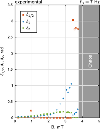
Figure 10. Angle oscillation amplitudes during rotation for B from 0 to 5 mT at a frequency fB = 7 Hz. δ1 is the amplitude of the oscillation at ωB, δ2 is for oscillation at 2ωB, δ1/2 is for oscillation at ωB/2.
Download figure:
Standard image High-resolution image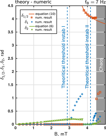
Figure 11. Angle oscillation amplitudes during rotation for B from 0 to 5 mT at a frequency fB = 7 Hz. δ1 is angle oscillation at ωB, δ2 is angle oscillation at 2ωB, δ1/2 is angle oscillation at ωB/2. Crosses, circle and square for measurements. Orange line for analytical solution equation (3). Green dashed line for simulation. Note that δ1 and δ1/2 from simulations are too small to be visible on the graph.
Download figure:
Standard image High-resolution imageRotation regime has its mode 2 oscillations described by equation (6). Simulation shows that δ2 has a completely different behavior for B > 6.2 mT at 10 Hz and for B > 3.2 mT at 7 Hz. This is happening with the growth of a first harmonic oscillation. To explain this change of dynamics, we investigate the nonlinear terms of equation (4) since the oscillations are not negligible anymore compared to the drive. As this first harmonic growth appears at high magnetic field, we simplify equation (4) considering  ,
,  and a solution sets as
  . One gets:

It is a parametric instability equation. Using the Laplace variation method, one gets the following solution:
The dispersion relation equation (9) indicates that the mode 1 can grow if k2 is a positive real. Solving equation (9) indicates a magnetic field threshold of 2.8 mT for fB = 7 Hz and 5.8 mT for fB = 10 Hz. This corresponds to the numerical measurements (figures 10 and 5) and to the experimental results (figure 10) despite a slight overestimation of the experimental threshold. This may be explained by the presence of the mode 1, even for the simple rotation regime: the experimental setup has a sub-milimetric excentration.
Regime 1/2 oscillation layer appears suddenly with a very sharp magnetic threshold. As a fist analysis, we define the existence condition of this regime by setting  in equation (1), using the Jacobi–Anger development and neglecting the friction. The solution for this regime is then:

where Jν(z) is the Bessel function of the first kind. This amplitude is reported in figure 11 with a very good agreement. The comparison to the experimental measurements is not so good, we recover the magnitude order and the tendency. Equation (10) does not have a solution for every value of the magnetic field for a given frequency fB: it requires a magnetic field greater than 3.7 mT at 7 Hz. Then, both rotation regime and mode 1/2 oscillation regime are possible in this parameter space ![$[B,{f}_{B}]$](https://content.cld.iop.org/journals/1402-4896/94/1/015002/revision2/psaaecf3ieqn12.gif) region. It is not mathematically proved, but experimentally, the oscillating regime is always dominating the rotation one.
region. It is not mathematically proved, but experimentally, the oscillating regime is always dominating the rotation one.
As for the rotation regime, the 1/2 oscillation mode has a change of behavior of its amplitude δ1/2 that appears with the increase of a mode 1 oscillation. Here again, we set the first mode as a small fluctuation:  . We still neglect friction and recover a parametric equation:
We solve it again with the Laplace variation method. The second right hand side terms do not provide any contribution to the mode 1. The first right hand side term leads to the dispersion relation:
Mode 1 is unstable if k2 is a positive and real. The magnetic field threshold is equal to 8.5 mT at fB = 10 Hz, which is out of the range of our experimental setup. At fB = 7 Hz, it is 4.2 mT: this value is recovered numerically, figure 11. There is a larger error of 0.5 mT with the experiment. If the calculus of the instability threshold is done with the experimental value of δ1/2 ≃ 3 rad, we obtain 3.8 mT which provides a much better agreement with experimental data. This validates the parametric instability mechanisms.
Two elements remain unexplained here. The first is the prevalence of the oscillating regime over the rotation regime for B > 3.7 mT at fB = 7 Hz as we said previously. The second is the chaotic dynamics that develops abruptly after the regime 1/2 oscillation pumped a mode 1 oscillation. This may be relative to the three period theorem [10]: the system can possibly exhibit the mode 1/2, 1 and 2 and then becomes chaotic, but this hypothesis is to handle with care.
6. Acceleration limit
There is an other limitation to the rotation regime which is not reported in figure 6. Experimentally, the compass lose its rotation at high speed long before the friction limit. This rotation loss is delayed if the frequency enhancement is done slowly. There is a link between the initial condition of the compass and the possibility of getting a rotation regime. To prove this acceleration limitation, we measure numerically and experimentally the possible frequency acceleration of the compass. The experiment consists in several simulations of equation (1) with fB = 25 Hz, B = 0.75 mT and various initial condition θi, ωi. Those simulations are confirmed by measurements: the same magnetic field is triggered for various initial conditions. Figure 12 gathers the cases where the rotation fails (white background or red crosses) or holds (gray background or blue circle). All the initial conditions do not reach a rotation regime. The compass needs enough kinetic energy and a constructive phase shift with the magnetic field, centered around ϕ = −π/2, in gray in figure 12. Each magnetic field defined by fB and B has an acceptance area around ϕ. Then the compass moves in the (θi, fi) graph and reaches its stationary state at (ϕ, fB).

Figure 12. Rotation or damped regime for a magnetic field with  , B = 0.75 mT and initial angle θi from −π to π and an initial speed from 10 to 40 Hz. Gray–white background are simulation results, Crosses and circles and experiment results.
Download figure:
Standard image High-resolution imageFigure 12 depends on fB and B. Then, to accelerate the compass and make a jump from  to
to  , we need
  to be in the acceptance area (gray zone) of the acceptable initial conditions graph for
  . This condition limits the value of the frequency jump. Moreover, the acceptance area shrinks while 1/B and fB increase: it is more and more difficult to reach the maximum speed set by equation (3). To illustrate this feature, we perform simulations estimating the maximal frequency jump Δf possible versus fB at the fixed phase ϕ and fixed B. Result are reported in figure 13 in colored lines for different magnetic field amplitudes. Δf tends to zero while the rotation frequency reaches its maximal value (equation (3), the stars in the figure at the bottom of each lines). This figure also shows the experimental results. We perform successive constant jumps from 10 Hz to the maximum speed reachable. For each jump, phase was kept constant, as the amplitude of the magnetic field which was fixed to 1 mT. This was repeated for Δf = 5, 4, 3 and 1 Hz. As expected, the rotation fails when the experimental Δf gets close or exceeds the maximum jump possible (the black bold line).

Figure 13. Color lines: maximal possible frequency jump Δf that keep the rotation for each frequency fB and for several B. ⋆: maximal possible frequency defined by equation (3). Black horizontal lines: experimental frequency jumps that keeps the rotation.
Download figure:
Standard image High-resolution imageIn practice, to reach a point in ![$[B,{f}_{B}]$](https://content.cld.iop.org/journals/1402-4896/94/1/015002/revision2/psaaecf3ieqn19.gif) , it is more time efficient to make large jumps at high magnetic field and then decrease the magnetic field to the wanted point: indeed, the variations of ϕ with the magnetic field are weaker. But this path is limited, by the magnetic field production which decreases with its frequency. Jumps to accelerate the compass must be smaller as the frequency increases and they must be done slowly to wait for the equilibrium between each jump.
, it is more time efficient to make large jumps at high magnetic field and then decrease the magnetic field to the wanted point: indeed, the variations of ϕ with the magnetic field are weaker. But this path is limited, by the magnetic field production which decreases with its frequency. Jumps to accelerate the compass must be smaller as the frequency increases and they must be done slowly to wait for the equilibrium between each jump.
7. Conclusion
This work relates complementary results on the bipolar motor used for chaos determination. It provides information on compass locking, rotation or oscillation regimes, such as their location in the parameter space ![$[B,{f}_{B}]$](https://content.cld.iop.org/journals/1402-4896/94/1/015002/revision2/psaaecf3ieqn20.gif) . All the presented results are supported by measurements, simulations and computations all in good agreement. The surprising presence of parametric instabilities in the periodic regimes was for the first time explored and is probably involved into the chaos generation. We have observed that the chaotic region of the parameter space is in fact an alternation of periodic regimes with chaotic ones, forming a diagram in layers. The complete structure of the parameter space may contain other layers, especially with a system with less friction and with a better experimental resolution which are unaccessible on our system because of a too high friction coefficient of the compact axis.
. All the presented results are supported by measurements, simulations and computations all in good agreement. The surprising presence of parametric instabilities in the periodic regimes was for the first time explored and is probably involved into the chaos generation. We have observed that the chaotic region of the parameter space is in fact an alternation of periodic regimes with chaotic ones, forming a diagram in layers. The complete structure of the parameter space may contain other layers, especially with a system with less friction and with a better experimental resolution which are unaccessible on our system because of a too high friction coefficient of the compact axis.
Appendix A.: Parameter definition
In this section, we will discuss the different methods used to measure each parameter. This is particularly important as it allows us to link experimental data with numeric simulations, and the different regimes rely deeply on the value of these parameters.
A.1. Magnetic moment
The magnetic field  generated by the compass is a function of
  . We can deduce its value by measuring
  for different distances z along the axis of the magnetic moment:

This law is only verified for large distances compared to the compass' size.
We obtain (figure A1):

Figure A1. Calibration of the magnetic moment  .
.
Download figure:
Standard image High-resolution imageA.2. Moment of inertia
For a constant magnetic field and small oscillations ( ) of
) of  , the differential equation can be rewritten as:

And the oscillation period is:
We measure the frequency for several values of  and the slope gives us the moment of inertia (figure A2):

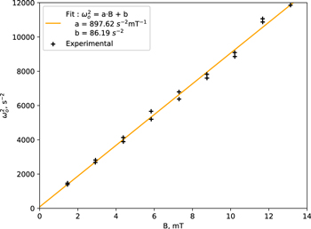
Figure A2. Calibration of the moment of inertia J.
Download figure:
Standard image High-resolution imageA.3. Coefficient of friction
Shuting down the magnetic field while the compass is oscillating at a constant speed (50 Hz) allows us to get the value of the friction coefficient. The differential equation verified by  becomes:

Therefore, speed decreases exponentially (figure A3) and we get:


Figure A3. Calibration of the coefficient of friction F.
Download figure:
Standard image High-resolution imageAppendix B.: Code description
B.1. Code algorithm
In order to properly sort every regime according to the magnetic amplitude  and frequency fB, we numerically resolve the equation of motion for different values of
  and fB, as an initial value problem. Several functions are used.
- a.Resolution: takes in parameters the initial conditions (θi, fi),
 and fB and returns θ(t) and .
 - b.Regime: takes in parameters θ(t) and and returns a string corresponding to the regime: 'Damped', 'Oscillation', 'Rotation' or 'Chaos'.
- c.RegimeMap: takes in parameters the maximal frequency and amplitude of the magnetic field, the resolution in frequency res(fB) and in amplitude . It returns a matrix of size representing the regime evolution with and fB.
- d.The parameters of simulations are located as following:


B.2. Dynamics sorting algorithm
Dynamics sorting in the function regime follows the algorithm represented in figure C1.
First damped motion, where  and
and  , is eliminated. Then, we compare values of θ(t) and
  on two time intervals I1 = [t1, t2] and I2 = [t2, t3]. If
  stays constant on these intervals, the regime is considered as an oscillating one. Finally, if
  stays constant on these intervals but
  evolves, the regime is considered as a rotating one. Every other regime is considered to be chaotic.
Appendix C.: Convergence study
In order to properly map every regime, it is important to choose a precise enough step size so that a regime is not mistaken for another. The relevant time scales of the equation are TB (the period of the magnetic field) and T0 (the fundamental period for the oscillation regimes,  ). To properly resolve the trajectory of the compass, we must choose :

Therefore the sampling frequency must depend on these parameters. Even when these conditions are respected, there is still some indetermination on the resolution of the trajectories, as the system can develop harmonics at higher frequencies (as with the small oscillations during rotating regimes).
Furthermore, as some regimes are chaotic and thus deeply dependent on initial conditions, it is impossible to get the real analytic solutions with a discrete time step.

Figure C1. Algorithm used for regime detection.
Download figure:
Standard image High-resolution imageIndeed, as seen on figure C2, a small error due to resolution issues will increase and the numerical solution will diverge from the analytic one: the longer you wait, the more precise you have to be. Therefore, we used a step size of 0.0001 s to ensure that our regime map was properly resolved during the characteristic time of the simulation.

Figure C2. Numerical solutions θ(t) for different step sizes in chaotic motion.
Download figure:
Standard image High-resolution image