


Abstract
Solid State Ionics has its roots essentially in Europe. First foundations were laid by Michael Faraday who discovered the solid electrolytes Ag2S and PbF2 and coined terms such as cation and anion, electrode and electrolyte. In the 19th and early 20th centuries, the main lines of development toward Solid State Ionics, pursued in Europe, concerned the linear laws of transport, structural analysis, disorder and entropy and the electrochemical storage and conversion of energy. Fundamental contributions were then made by Walther Nernst, who derived the Nernst equation and detected ionic conduction in heterovalently doped zirconia, which he utilized in his Nernst lamp. Another big step forward was the discovery of the extraordinary properties of alpha silver iodide in 1914. In the late 1920s and early 1930s, the concept of point defects was established by Yakov Il'ich Frenkel, Walter Schottky and Carl Wagner, including the development of point-defect thermodynamics by Schottky and Wagner. In terms of point defects, ionic (and electronic) transport in ionic crystals became easy to visualize. In an 'evolving scheme of materials science', point disorder precedes structural disorder, as displayed by the AgI-type solid electrolytes (and other ionic crystals), by ion-conducting glasses, polymer electrolytes and nano-composites. During the last few decades, much progress has been made in finding and investigating novel solid electrolytes and in using them for the preservation of our environment, in particular in advanced solid state battery systems, fuel cells and sensors. Since 1972, international conferences have been held in the field of Solid State Ionics, and the International Society for Solid State Ionics was founded at one of them, held at Garmisch-Partenkirchen, Germany, in 1987.
Export citation and abstract BibTeX RIS

Content from this work may be used under the terms of the Creative Commons Attribution-NonCommercial-ShareAlike 3.0 licence. Any further distribution of this work must maintain attribution to the author(s) and the title of the work, journal citation and DOI.
1. Introduction
By definition, Solid State Ionics is concerned with the motion of mobile ions in the solid state. This discipline encompasses a remarkably wide range of themes in both basic science and applications.
In basic science, the central themes are about the equilibrium and non-equilibrium characteristics of disordered ionic materials. On a microscopic level, the thermodynamic and transport features largely result from the disordered structures of the materials under consideration. This includes their equilibrium properties such as the microscopic ion dynamics in them as well as their non-equilibrium properties such as the microscopic and macroscopic flows of mass and charge in potential gradients, and, finally, chemical reactions in the solid state.
The insights gained in the field of basic science provide ample possibilities for finding novel materials and devices for applications, in particular for those that help us to preserve our environment by cleaner, smarter and more efficient ways of energy conversion and storage. High technology applications include, for instance, advanced solid state battery systems and a variety of fuel cells and chemical sensors.
Currently, the main endeavor of Solid State Ionics is to create connections, bridges, routes leading from basic science on the one hand to clean-energy technologies on the other. This is why, at the present time, Solid State Ionics appears more fascinating and flourishing than ever.
In search of the roots of Solid State Ionics, we need to trace the above scientific and applied themes back to their origins, which leads us to those who laid the foundations. Many names come to mind, possibly starting with Luigi Galvani and Alessandro Volta. In the decades and centuries to follow, the most eminent names include those of Michael Faraday, Walther Nernst and Carl Wagner. They were the giants on whose shoulders we stand today.
At this point, it becomes evident that Solid State Ionics has its roots essentially in Europe. Pursuing the lines of development of the different themes of Solid State Ionics over time, from their discovery up to the present day, we must, therefore, start in Europe.
2. Michael Faraday (1791–1867)
Imagine going back in time to the first part of the 19th century. The laws of thermodynamics were still unknown, and even Ohm's law was not formulated until 1826. Nobody knew about the periodic structure of crystals, and concepts such as point disorder and how to express this phenomenon in terms of entropy were still one century away. It is also worth mentioning that even at the beginning of the 20th century, famous scientists such as Ernst Mach and Wilhelm Ostwald still refuted the very existence of atoms and ions.
Most admirably, the 'genius of Michael Faraday', as we rightly say today, discovered the motion of mobile ions in both liquid and solid electrolytes. This was achieved in a few years, from 1831 to 1834. He thus laid the foundations not only of electrochemistry but also of Solid State Ionics.
What information could Faraday build on when he succeeded Sir Humphry Davy as director of the laboratory of the Royal Institution in London, in 1825? In 1800, Alessandro Volta had constructed his famous electric pile, consisting of many consecutive plates of silver, zinc and cloth soaked in salt solution. In the same year, the English scientists William Nicholson and Anthony Carlisle used this pile to decompose water electrolytically into oxygen and hydrogen, and a few years later Humphry Davy himself discovered the elements sodium and potassium, isolating them by electrolysis with the help of a voltaic pile.
In his own studies of the decomposition of solutions by electric current, Faraday (figure 1) already used our present nomenclature, i.e., the terms ion, cation, anion, electrode, anode, cathode, electrolyte and electrolysis [1]. He was, indeed, the first to identify the passage of charge through an electrolyte with the motion of mobile ions and to discover the ability of ions to exchange their charges with an electrode when, in the process of electrolysis, they were liberated and transformed into the elements.
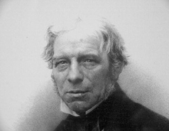
Figure 1. Michael Faraday, about 1860.
Download figure:
Standard image High-resolution imageMore quantitatively, he discovered what is now known as Faraday's first and second laws of electrolysis. His first law (1832) states that the mass of any product liberated at the electrode by electrolysis, Δm, is proportional to the quantity of electricity passed through the electrolyte, Δq. According to his second law (1833), the masses of products liberated in electrolysis by the same quantity of electricity are always proportional to an element-specific 'electrochemical equivalent'.
In his own words: 'Thus hydrogen, oxygen, chlorine, iodine, lead, tin, are ions; the three former [after hydrogen] are anions, and the two metals are cations, and 1, 8, 36, 125, 104, 58 are their electrochemical equivalents nearly'.
Denoting the (positive or negative) number of elementary charges, e, on an ion by z, we now realize that an 'electrochemical equivalent' is just the ratio of the molar mass, M , in g mol−1, divided by z . Therefore, the first and second laws imply Δ m ∝ Δ qM/z . This proportionality may be converted into an equation, F = (Δ q/Δ m)(M/z) , which specifies the total charge of univalent ions per mol, F ≈ 96 485 A s mol - 1 . Nowadays, F is called Faraday's constant or, as a unit, simply the faraday.
Michael Faraday was also the first to discover electrolytes that were not liquid, but solid. In 1834, he recorded the following observation [1]:
'I formerly described a substance, sulfuret of silver, whose conducting power was increased by heat; and I have since then met with another as strongly affected in the same way: this is fluoride of lead. When a piece of that substance, which had been fused and cooled, was introduced into the circuit of a voltaic battery, it stopped the current. Being heated, it acquired conducting powers before it was visibly red hot in daylight; and even sparks could be taken against it whilst still solid'.
As pointed out by Michael O'Keeffe [2] in 1976, 'this appears to be the first observations of the transition from the poorly conducting to the conducting states in ionically conducting materials that we now call solid electrolytes'. Today we distinguish between solids with mixed ionic/electronic conduction (MIEC), such as silver sulfide, and ionic conductors such as lead fluoride. Unaware of this difference, Michael Faraday discovered the first members of these two classes as early as in 1834.
Lead fluoride, PbF2, is the archetype of those solid electrolytes in which the transition into the highly conducting state is not of first order, but appears to be continuous and spread out over a temperature range of typically 100 K or more. This kind of transition is now termed 'Faraday transition' [2], after its discoverer. Cation conductors that show a Faraday transition include Na2S and Li4SiO4, while anion conducting crystals displaying the same property are, for instance, PbF2, CaF2, SrF2, SrCl2, with the fluorite structure, and LaF3, with the tysonite structure.
The variations of heat content and ionic conductivity as observed in the course of the Faraday transition of PbF2 are shown in figure 2 [2, 3]. The peculiar shape of the temperature-dependent heat content is equivalent to a specific heat with a broad maximum around and below 700 K. It reflects a continuous increase of the degree of disorder in this temperature range, which results in a correspondingly rapid increase of the ionic conductivity.

Download figure:
Standard image High-resolution image3. Toward Solid State Ionics: early lines of development
When it comes to characterizing ionic conduction in solids, i.e. to answering the basic questions of Solid State Ionics, we can these days build on a solid background of knowledge, and we can rely on experimental techniques that are readily available. The relevant pieces of information that we expect to obtain always include 'the how and the why'. More explicitly: (i) How do the mobile ions move locally and translationally, resulting in unusually high values of diffusivity and conductivity? (ii) Why is it possible for them to move so easily, i.e. why does the disordered structure provide sufficiently low energy barriers for their hopping motion?
Asking all these questions, we normally do not notice that even the very terms and concepts that we use, such as 'conductivity', 'diffusivity', 'structure' and 'disorder' have been developed only during the past two centuries and, indeed, that this has essentially been done in Europe. In this section, we will sketch those early lines of development, which paved the way for the emergence of Solid State Ionics in its present form.
3.1. Linear laws of transport
In 1826, the German physicist Georg Simon Ohm realized that the electric current through a conductor between two points, I , is directly proportional to the electric potential difference between these points, U . This linear law, now known as Ohm's law, may be expressed as U = RI , where R is the resistance of the conductor. The unit for R , denoted by the Greek letter Ω , is now called an ohm.
In his 1827 paper [4], Ohm pointed out that his law of charge transport was quite analogous to the law of heat conduction discovered by Joseph Fourier in France in 1822 [5]. Indeed, both linear laws relate a flux density,  , to a 'driving force',
  , which is a negative gradient of a 'potential',
  . Note that vectorial quantities or operators are underlined. In the case of heat conduction, the 'potential', φ , is temperature, T , while for charge transport it is the electrical potential. Denoting the flux density of electric charge by
  and the electric field by
  , one may now introduce the electric conductivity, σ , and thus write Ohm's law as
  .
.
The third law in this series is Fick's first law of diffusion, discovered by Adolf Fick in Germany in 1855 [6]. In Fick's first law,  , the notations
  , D and n represent the particle flux density, the diffusion coefficient and the number density of the particles, respectively. This linear law, when combined with the continuity equation, yields Fick's second law, which describes the development of the number density in space and time and thus provides the basis for deriving diffusion coefficients from experimental data obtained under different kinds of boundary conditions [6].
In understanding diffusion, a big step forward could be made, once the American Josiah Willard Gibbs had discovered the concept of the chemical potential, μ, in 1878 [7]. It then became obvious that the driving force for 'chemical' diffusion of a mobile species was in fact not  , but rather the negative gradient of its chemical potential,
  , with
  . In this expression, μ° and kB are the standard chemical potential and the Boltzmann constant, respectively. The activity, denoted by a , becomes identical with n/n° only in the ideal case. This particular case implies
  , and Fick's first law is thus recovered.
Historically, the next step forward was to introduce the so-called electrochemical potential of an ion, η, via η = μ + qφ. Here, q = ze is the ionic charge. It thus became possible to formulate one linear law, combining diffusion and conduction, by writing  . In essence, this is the line of thought pursued by Walther Nernst in Germany around 1888 [8]. The Nernst–Planck equation,
  , was thus obtained for particles that carry charge q and follow the ideal law. Also, the famous Nernst–Einstein relation, σ = D(nq2/kBT), was now readily derived, which could be done by multiplying the Nernst–Planck equation by q on either side and then identifying its conduction term with
  .
.
Under the general heading of 'mobile charge carriers', three more milestones were accessed in the second half of the 19th century, all of them in Europe. Remarkably, they may all be considered continuations of the work of Michael Faraday. Two of them concern the identity of charge carriers, while the other one is the extension of the concept of conductivity to non-zero frequencies.
- (i)In 1881, Hermann von Helmholtz deduced from Faraday's laws of electrolysis that electricity itself was probably particulate, thus anticipating the very concept of the electron [9].
- (ii)
- (iii)In 1861, James Clerk Maxwell took up Faraday's concept of fields and introduced the displacement field,
 [12]. In a sample, the time derivative of this quantity may be identified with the flux density of the electric current, . This concept is most useful, if the sample is exposed to an electric field that varies periodically with angular frequency ω, written (in complex notation) as . The displacement field in the sample is then , where and ε0 are its complex dielectric function and the vacuum permittivity, respectively. After differentiation of the displacement field with respect to time Ohm's law is recovered in the form of , with . Nowadays, broadband conductivity spectra of solid electrolytes can be measured over more than 17 decades, providing valuable information about the dynamics of the mobile ions.


3.2. From Faraday to von Laue: an avenue toward structural analysis
Why should atoms or ions be mobile in a solid, thus opening up the possibility of translational transport? Clearly, this is impossible in a perfectly ordered crystal. Rather, ionic motion and transport require a defective structure of the material under consideration.
If the material is a glass, the arrangement of the ions does not display the property of long-range order. Within this glassy structure, it is then possible to visualize the existence of unoccupied sites, which the mobile ions can use for their hopping motion.
If the material happens to be, for instance, the high-temperature phase of silver iodide or silver sulfide, then the entire silver sublattice is effectively molten and, therefore, ionically conductive.
In most cases, however, the material under consideration will have a more or less regular crystal structure that contains a large number of defects, mostly point defects, which serve as vehicles for the motion of mobile ions. In this case, there are two steps to go. The first essential step is to determine the basic crystal structure itself, while the second is to identify the defects contained in it.
In this subsection, we consider the first of these steps, because there is a remarkable historical avenue of progress explored exclusively by European physicists. It starts out from Michael Faraday's work and eventually leads to the Nobel Prize in Physics rewarded to Max von Laue in 1914 and, later, to all those techniques of structural refinement that are indispensable for us today.
We first recall that, in the 19th century, crystals were generally classified by their outer appearance only, which led to the introduction of Miller indices in 1839 and of Bravais lattices in 1845. However, there was still no experimental proof for the strictly periodic arrangement of atoms or ions in crystals, constituting the essential feature of long-range order.
Remarkably, the roots for the novel breakthrough approach were in essence laid by Michael Faraday, who not only introduced the field concept to describe, for instance, the magnetic field lines accompanying an electric current, but also discovered the phenomenon of electromagnetic induction. In 1861, James Clerk Maxwell built on Faraday's ideas and observations when formulating his famous 'Maxwell equations' [12]. Four years later, Maxwell constructed a wave equation from them, describing the variations in space and time of electric and magnetic fields that form a wavelike pattern [13]. To his own surprise, he realized that this wavelike pattern would move in a vacuum with the known speed of light,  , where μ0 denotes the vacuum permeability. He was thus struck by the insight that light waves were, indeed, electromagnetic waves. In 1887, Heinrich Hertz proved experimentally that the same was true for radio waves.
The second essential ingredient on the way toward structural analysis was the discovery of x-ray radiation by Wilhelm Conrad Röntgen in 1895 (Nobel prize in physics, 1901). To indicate that this type of radiation was completely new, he referred to it simply as 'X'.
As it were, the above ingredients were luckily combined in the mind of Max von Laue in the winter of 1911/1912, when he took a walk with Paul Peter Ewald through the English Garden in Munich. It was then that he considered the possibility that x-rays might be electromagnetic waves as formulated by Maxwell, but with a much shorter wavelength than visible light. If they had the proper wavelength, they might be diffracted by the atoms in a crystal, just like visible light is diffracted by a much wider grating. Shortly afterward, his idea was corroborated experimentally, with the following consequences:
- (i)X-rays are, indeed, short-wavelength electromagnetic waves.
- (ii)Crystals are composed of atoms or ions displaying lattice periodicity.
The techniques pioneered by Max von Laue were further developed by Sir William Henry Bragg and his son, William Laurence Bragg, who were awarded the Nobel Prize in Physics immediately after Max von Laue, in 1915. Since those early days, x-ray diffraction has been more and more perfected and has become the method of choice for structural analysis of crystalline (and non-crystalline) matter.
3.3. Disorder in solids: thermodynamics and the role of entropy
As mentioned above, disorder is a prerequisite for ionic transport in any solid electrolyte. However, the task of elucidating the type and degree of the specific disorder that is present in a given crystalline material at a given temperature is much more demanding than ordinary structural analysis.
Nowadays, structural refinements on the basis of x-ray (or neutron) diffraction experiments are quite important in determining disordered structures and the possibilities for mobile ions to move in them. Lead fluoride, see figure 2, provides an excellent example. In this case, the maximum of the heat capacity near 700 K, which is indicative of an order–disorder transition, could be explained in a detailed neutron-diffraction study of structural changes that result in an increase of the mobility of the mobile fluoride ions, and hence of the ionic conductivity, with increasing temperature [14]. While this kind of study became possible in the late 20th century, similar investigations were of course out of the question in the early days of x-ray diffraction.
Historically, the route toward a quantitative understanding of disorder in crystals, and especially of point defects, was quite different. The foundations for the relevant insights were, in fact, laid by the advent of thermodynamics and, in particular, by the notion of the role of entropy.
Since Faraday's time, it had been known that ionic conductivities of solid electrolytes generally increased with increasing temperature. If this happened in a well-defined and reproducible fashion, this might well reflect a concomitant increase of the degree of disorder. Over time, such considerations led to the view that disorder should, indeed, be regarded as a temperature-dependent equilibrium property, to be treated in terms of equilibrium thermodynamics.
In retrospect, we now realize that it was this approach that eventually led to the formulation of point-defect thermodynamics by Carl Wagner and Walter Schottky from 1929 onward [15–19]. In their rigorous statistical treatment, the interrelationship between disorder and entropy was of prime importance, see the pertinent section below. Of course, Wagner's and Schottky's work had become possible only by the thorough understanding of entropy that had been attained during the decades before. On the way toward this understanding, the following stages of development appear most significant. They are associated, essentially, with the names of Rudolf Clausius, Ludwig Boltzmann, Walther Nernst and Max Planck.
- (i)In 1865, Rudolf Clausius formulated the change of entropy of a sample, dS, as the ratio of the heat that was absorbed reversibly, dQ, by temperature. For the case of isobaric heating, it thus became possible to express not only dH = Cp (T)dT, i.e. the change in enthalpy, but also the change in entropy, dS = (Cp(T)/T)dT, in terms of the heat capacity of the sample at constant pressure, Cp (T). Therefore, specific heat measurements became increasingly important for the construction of thermodynamic functions such as enthalpies and entropies, as well as Gibbs energies, G = H-TS.
- (ii)Ludwig Boltzmann's historical merit was in discovering the statistical meaning of thermodynamic functions. If, for example, the macroscopic state of a closed system is consistent with W different microstates (quantum states in modern language), then its entropy will be. This is the famous Boltzmann equation, with the Boltzmann constant, kB. On his tomb stone at Vienna, it is engraved in the form . The generalized meaning of this equation for solids, liquids and gases was pointed out by Max Planck around 1900. Here it is interesting to note that, in deriving the equation, an additive constant (appearing on integration) was set equal to zero, thus yielding S = 0 for the special case of W = 1, see below.
- (iii)In 1905, Walther Nernst established what he called 'My Heat Theorem', later known as the Third Law of thermodynamics (Nobel prize in chemistry, 1920). The idea came to him during a lecture at the University of Berlin (now called Humboldt University), and a bronze plaque still marks the place where this happened. Nernst realized that, for pure homogeneous phases in thermal equilibrium, the internal energy, U(T), and the Helmholtz (free) energy, A(T) = U(T)-TS(T), did not only approach the same value for, but did so with their first derivatives becoming zero in this limit. As an immediate consequence, the entropy of such phases, S(T), must approach zero in the limit of . This stronger statement was made subsequently by Max Planck in 1910.


Important conclusions can be drawn from (i) to (iii). Firstly, the proper value of the entropy of a sample is, indeed, obtained by taking the integral (which exists) over (Cp (T)/T)dT from zero temperature upward. Secondly, the same value is also obtained by inserting the number of possible (quantum) states, W, into the Boltzmann equation, with  for ordered equilibrium phases in the limit of very low temperatures.
During the years from 1876 to 1878, Josiah Willard Gibbs had shown that, at given values of pressure and temperature, the equilibrium state of a sample is the one in which its Gibbs energy, G = H -TS, attains a minimum [7]. Large values of S are thus increasingly favored at high temperatures, and the function W(T) must, therefore, be rapidly increasing. In an ionic crystal, the number of possible arrangements of the ions is hence expected to become larger and larger as temperature is increased, corresponding to more and more disorder in the crystal lattice. In thermal equilibrium, higher temperatures thus give rise to higher degrees of disorder and, hence, to higher ionic conductivities, in agreement with experimental evidence. The increase in disorder and conductivity may be gradual as in lead fluoride or it may occur in a first-order phase transition as in silver iodide. The latter was discovered by Tubandt and Lorenz in 1914 [20], see below.
3.4. Electrochemical storage and conversion of energy
In the 19th century, it became apparent that different kinds of energy, such as heat, mechanical work and electrical work, were equivalent and could be transformed into each other, provided the first and second laws of thermodynamics were not violated. Known devices for energy conversion included the heat engine and the heat pump, the electric motor and the dynamo machine. The notion of equivalence between the abovementioned energies also triggered the definition of respective energy units that are all identical, i.e. 1 Joule (J) = 1 Newton ⋅meter (N m) = 1 Watt ⋅second (W s).
A further equivalence is the one between electrical and chemical energy, which is considered and exploited in electrochemistry. To mention an early example of an electrochemical process, let us recall the work of William Nicholson and Anthony Carlisle who applied a voltage to decompose liquid water into the gases hydrogen and oxygen. The electrolysis of water was thus discovered as early as in 1800. However, it took almost one more century until the basic principle was understood, i.e. that the electric energy consumed and the chemical energy taken up in the reaction were, indeed, identical.
In 1838, the reverse step was performed by the German scientist and inventor Christian Friedrich Schönbein and a year later by William Robert Grove in England [21]. They constructed devices in which the gases hydrogen and oxygen combined to form water, thereby producing electricity—the first fuel cells.
In a fuel cell, chemical energy may be provided (and then converted) continuously by suitable flows of those gases that are required for the reaction. By contrast, a galvanic cell or battery can store and discharge only a limited fixed amount of energy. Upon charging and discharging, this energy is, respectively, transformed from its electric state into its chemical state and vice versa. Note that, in common usage, the word 'battery' has come to include a single galvanic cell, although a battery properly consists of multiple cells.
The archetypal galvanic cell, now called the Daniell element, was introduced by John Frederic Daniell in England, in 1836. It consisted of two half cells, one with a zinc pole in a solution of zinc sulfate, the other with a copper pole in a solution of copper sulfate. This cell was free from polarization and could maintain a steady voltage.
About two decades later, Gaston Planté invented the lead acid battery, which he demonstrated to the French Academy of Science in 1860. Owing to its robustness and reliability, this battery has been used up to the present day, in particular for automotive starting, lighting and ignition. In spite of many improvements, the lead acid battery still has its characteristic shortcomings, i.e. it is heavy, bulky and poisonous. Therefore, a replacement by more lightweight, yet highly efficient solid state battery systems is now overdue. This is, indeed, one of the topical challenges of Solid State Ionics, while the optimization of all-solid-state fuel cells constitutes another.
By the end of the 19th century, an understanding of the processes occurring in fuel cells and galvanic cells was eventually achieved, in particular by Wilhelm Ostwald and Walther Nernst.
The very term 'fuel cell' was coined by Wilhelm Ostwald. In his 1894 paper, he described the energy conversion in a fuel cell and especially emphasized the fact that its efficiency was not limited by the maximum efficiency of a reversible Carnot cycle [22]. In contrast to a heat engine, there was, therefore, no need for attaining high temperatures in the 'fuel cell combustion process'. Ostwald also noted that mobile ions had to move throughout the electrolyte (liquid or solid), from one electrode to the other. The reacting gases were thus separated, which prevented immediate explosion, but nevertheless allowed the reaction to proceed in a controlled fashion.
At that time, Wilhelm Ostwald, who was one of the founding fathers of electrochemistry (Nobel Prize in Chemistry, 1909), had essentially invented modern chemical ionic theory. Together with Svante Arrhenius and Jacobus Henricus van't Hoff, he formed a group that was called 'The Ionists' and continued making progress in their field.
In the years to follow, however, Ostwald surprisingly no longer adhered to the view that the concept of ions should be connected with a corpuscular picture. Instead, he turned to a philosophy of chemistry where, as described in his 1907 treatise Prinzipien der Chemie, he found no place for any 'hypothetic' sub-microscopic particles, and was thus clearly anti-atomistic [23].
The route taken by Walther Nernst, to be described in the next section, was based on the abovementioned equivalence of chemical and electric energies and led him to the creation of modern electrochemistry. His new formulation of this branch of science and technology enabled him to quantify the electric potential differences between the electrodes of any electrochemical cell (fuel cell or galvanic cell, the electrolyte being liquid or solid). This is the essence of his famous 'Nernst equation', which is still the most prominent single equation in the entire field of Solid State Ionics.
4. Walther Hermann Nernst (1864–1941)
Walther Nernst (figure 3) founded the Institute of Physical Chemistry at Göttingen in 1895 and was its director until 1905, when he moved to Berlin. His fundamental contributions to the science and technology of ionic transport in solids include the derivation of the Nernst equation and the detection of ionic conduction in heterovalently doped zirconia, which he utilized in his Nernst lamp and which has remained a 'high-tech' oxygen-ion conductor up to the present day.
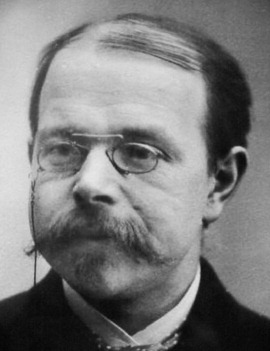
Figure 3. Walther Nernst, about 1895.
Download figure:
Standard image High-resolution imageHalf a century after Michael Faraday's seminal work in electrochemistry, Walther Nernst was inspired by Svante Arrhenius' dissociation theory [24], which emphasized the importance of ions in solution. At that time, the stage was thus set for reaching a more profound understanding of the theory of galvanic cells. Remarkably, this goal was attained by Walther Nernst as early as in 1889, during his time as a post-doctoral fellow under Friedrich Kohlrausch, at the University of Würzburg [25].
The new point of view was to regard the processes happening in electrochemical cells as chemical reactions that involved charged species as reaction partners. Was it possible to extend the thermodynamic treatment of chemical reactions, developed earlier by Gibbs, into a corresponding electrochemical theory? Here, Walther Nernst's outstanding scientific merit was in realizing that electrochemical equilibria could be formulated in analogous fashion to chemical equilibria, if the chemical expressions were suitably complemented by their electrical counterparts. Electrochemical equilibrium could then be defined in terms of a minimum principle for the sum of the total chemical and electrical energies of the system. This implied a balance in the sense that any variations of these energies must compensate each other, thereby reflecting their equivalence.
The essence of Nernst's treatment of electrochemical equilibria is best outlined in terms of the chemical and electrochemical potentials of the reacting components, which are written as  and ηi = μi + zi Fφi, respectively. These are now molar potentials, differing from the ones used earlier (in the subsection on linear laws) by the replacement of kB T with RT and of qi = zi e with zi F. As usual, the stoichiometric coefficients, νi, are in the following taken to be positive for the products and negative for the educts.
In terms of chemical potentials, the condition for chemical equilibria is most conveniently written as 0 = ∑ νi μi, which corresponds to a minimum of the Helmholtz (free) energy of the system, A, if temperature and volume are kept constant, and to a minimum of its Gibbs energy, G = A + pV , if temperature and pressure are kept constant. This was of course well known to Nernst [8], although he only rarely used chemical potentials.
In a similar fashion, Nernst's view of the condition for electrochemical equilibria is most clearly conveyed by a new identity, which is 0 = ∑ νi ηi. Evidently, this sum consists of a chemical term, ∑ νi μi, plus an electric term, ∑ νi zi Fφi. The electric potential difference in the cell, by convention written as E = φright - φleft, is traditionally called the electromotive force (e.m.f.). In terms of E, the electric term becomes |z|FE, where |z| is the number of charges exchanged at the electrodes in an elementary process. As pointed out by Nernst, this quantity, |z|FE, is the maximum amount of electric work that can be obtained from the cell, upon reversible discharging [8].
The chemical term is, more explicitly,  . It may be identified with the molar change in Gibbs energy, Δ Gm, if temperature and pressure are kept constant. The following identities, Δ Gm ° = ∑ νi μi ° and
  , are used in a further step, and it then becomes obvious that, in electrochemical equilibrium, the terms Δ Gm °,
  and |z|FE must add up to zero. Introducing the standard e.m.f. of the cell, E° = - Δ Gm°/(|z|F), one now obtains the famous Nernst equation
Applying this equation, Walther Nernst was the first to reproduce e.m.f. data successfully, and he did so for many different types of electrochemical cells that all contained liquid electrolytes [8]. In his own work, however, Nernst did not use activities. He rather argued in terms of an 'electrolytic pressure of dissolution' that was assumed to force ions from electrodes into solution. He was thus led to use normalized pressures, pi /p°, and normalized concentrations, ci /c°, instead of activities. A further approximation he often made was to employ Helmholtz energies instead of Gibbs energies, arguing that the difference had little effect on the e.m.f.
Providing a quantitative connection between easily measurable voltages on the one hand and non-trivial thermodynamic data on the other, the Nernst equation has, over the decades, proved invaluable for the field of Solid State Ionics, strongly spurring its further development.
In basic research, relevant thermodynamic properties of ion-conducting materials became experimentally accessible. One example concerns the significant changes in the activities of the mobile species that often accompany comparatively small compositional changes in solid electrolytes. These could now be determined, for instance, by utilizing the Nernst equation to evaluate coulometric titration data.
Most importantly, countless applications of ionic transport in disordered materials rely on the Nernst equation. These include all kinds of solid state devices for electrochemical energy conversion, such as fuel cells and advanced battery systems, as well as a multitude of chemical sensors that are used in technical processes and for the purpose of preserving our environment, e.g. in the lambda probe.
It is worth mentioning that Walther Nernst himself was always in search of ways to provide basic scientific knowledge for the advancement of new technologies and applications. An impressive example is his invention of the Nernst lamp, which was highly acclaimed as it produced overwhelmingly beautiful 'natural' light. By the end of the 19th century, Nernst thus perfectly met the strong public desire for bright electric light, which had emerged throughout Europe and the United States.
While Thomas Edison's incandescent light bulb, patented in 1879, contained a glowing carbon filament, Walther Nernst used a solid electrolyte, the so-called Nernst mass, see below, as an electrically conductive ceramic rod [26, 27]. The advantages thus achieved were twofold. Firstly, the Nernst lamp, patented in 1897, required no vacuum, but could be operated in ambient air. Secondly, its emission in the visible spectrum was brilliant and close to daylight.
One disadvantage was, however, that the ceramic rod was not sufficiently conductive at room temperature, so the Nernst mass had to be preheated to its operational temperature. In the original sketch of figure 4, a Bunsen burner was used for this purpose, while a separate heater filament was employed later. For heat protection, the main components were then enclosed in a glass bulb. These technical improvements date back to the years when Nernst had already sold his patent to AEG, the General Electric Company at Berlin, for 1 million Goldmark, which was quite a fortune at that time.
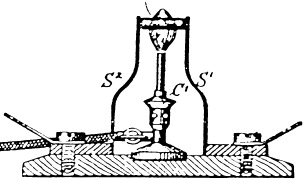
Figure 4. Original sketch of the Nernst lamp, with C' marking the Bunsen burner used for preheating, by courtesy of H Schmalzried.
Download figure:
Standard image High-resolution imageAlthough the Nernst lamps were successfully marketed by the turn of the century and the AEG pavilion at the World's Fair 1900 at Paris was spectacularly illuminated by 800 of them, they eventually lost out to the more efficient tungsten filament incandescent light bulb, a development that Nernst himself had probably foreseen.
Nernst was surely aware that his Nernst mass was a 'conductor of the second kind', i.e. a solid electrolyte. What he could not have known were the structural details of the material, the mobile species and the ionic transport mechanism. Answers to those questions were given only decades later, when it became obvious that the Nernst mass was a solid solution of oxides of heterovalent ions, such as calcium and yttrium, in zirconia [28]. For reasons of charge neutrality, the fluorite-type crystal lattice contains numerous oxygen vacancies, which serve as vehicles for effective oxygen transport. Because of this latter property, the Nernst mass is predestined for applications in robust devices that rely on the transport of oxygen ions. In fact, it has remained a 'high tech' material up to the present day, being successfully used in solid oxide fuel cells, oxygen sensors and oxygen pumps. What remains is admiration for the 'certainty of a sleepwalker' [29] with which Walther Nernst identified the extraordinary potential of his Nernst mass for useful applications.
During his time at the University of Berlin, from 1905 onward, Walther Nernst's work concentrated on thermodynamics, his most outstanding success being the discovery of the third law. Referring to the uniqueness of his personality, Albert Einstein once said, 'I have never met any one who resembled him in any essential way'.
5. The discovery and extraordinary properties of alpha silver iodide
The high-temperature phase of silver iodide, α-AgI, is often considered the archetypal solid electrolyte. The surprisingly unexpected properties of α-AgI were discovered by Carl Tubandt and E Lorenz at Halle (Germany) in 1914, on the occasion of their measurements of the electric conductivities of the silver halides AgCl, AgBr and AgI [20]. Their original plot is reproduced in figure 5.
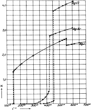
Figure 5. Ionic conductivity of the silver halides, original plot of Tubandt and Lorenz (1914) [20].
Download figure:
Standard image High-resolution imageNote that, throughout this text, Tubandt's notation for phases will be employed, denoting them by α, β, γ, etc in the order of their stability with decreasing temperature.
From the figure it is seen that AgI, in contrast to AgCl and AgBr, has a highly conducting solid phase—now known as the α-phase—stable between 147 °C and 555 °C. At the β to α phase transition, the conductivity of AgI increases by more than three orders of magnitude up to 1.3 Ω−1 cm−1. Within the α-phase, it increases only by a factor of two and then drops upon melting. The extraordinarily high value of the electrical conductivity of α-AgI and its relatively weak temperature dependence are comparable with those of the best conducting liquid electrolytes.
The discovery of α-AgI was the starting point for the investigation of a whole new class of optimized ion conductors, namely the so-called AgI-type solid electrolytes. In their early work, Carl Tubandt and his co-workers identified the following phases as belonging to this class: α-AgI, α-CuI, α-CuBr and β-CuBr, as well as the high-temperature phases of Ag2S, Ag2Se and Ag2Te [20, 30]. From their measurements of transport numbers and from their inter-diffusion experiments they concluded that in the highly conducting phases of the silver and cuprous halides the charge was carried by the cations [11, 30], whereas the silver chalcogenide phases were found to be mixed ionic and electronic conductors [31, 32]. Here we recall that the 'conducting power' of silver sulfide had already been discovered by Michael Faraday.
Since Tubandt's times, the Ag+ ions in α-AgI have been regarded as moving in a 'liquid-like' fashion within the crystallographic framework provided by the anions. A first structural analysis of α-AgI was presented by Strock (Germany) in 1934 [33] and 1936 [34]. On one hand, it was easy for him to assign a body-centered cubic (bcc) structure to the iodide sublattice. On the other hand, Strock encountered problems in localizing the silver ions. Trying to 'nail them down' crystallographically, he suggested three different kinds of partially occupied sites, totalling 6 + 12 + 24 positions for the two silver ions in the bcc unit cell. Of course, such a concept cannot grasp the liquid-like character of their arrangement and motion.
More than 40 years later, in 1977, the American scientists Cava, Reidinger and Wuensch used their single-crystal neutron-diffraction data to construct a contour map of the probability density of the silver ions in α-AgI,  [35]. The map shows flat maxima of
  at the tetrahedral voids and local minima at the octahedral positions. Saddle points occur between neighboring tetrahedral sites. It is, however, important to note that, except for the regions occupied by the anions, the variation of
  is relatively weak and smooth. At 250 °C, for example, the ratios ρ(tetrahedral site)/ρ(saddle point) and ρ(tetrahedral site)/ρ(octahedral site) are only two and three, respectively. Hence, one can conclude that the periodic potential barriers provided by the anions for the translational diffusion of the cations are only of the order of the thermal energy.
During the same decade, quasielastic neutron scattering experiments on poly- and single-crystalline α-AgI were performed at the Institut Laue-Langevin at Grenoble, France, in order to extract information on the local dynamics of the mobile silver ions [36]. The measured spectra were well fit by a model that approximates the actual Ag+ motion by a spatial convolution of two processes. One of them is a fast diffusive motion within a local cage of about 1 Å radius, while the other is a random hopping via tetrahedral positions. The former reproduces the almost isotropic broad quasielastic component, while the latter is in agreement with the shape and anisotropy of the narrower quasielastic line which is superimposed.
At about the same time, ionic Hall-effect data taken on α-AgI were perfectly explained by identifying mobility and Hall mobility of the silver ions and by assuming that, indeed, all of them were mobile in α-AgI [37]. The ionic conductivity of α-AgI was found to display no frequency dependence up to at least 40 GHz [38]. This implies that the mobile silver ions move so fast that any memory of individual movements is erased after a time which is the inverse of 2π × 40 GHz, i.e. after 4 ps.
6. The concept of point defects in ionic crystals
In contrast to the structural disorder and liquid-like motion of the silver ions in α-AgI, a quite different, much more solid-like state of affairs was encountered by Tubandt and Lorenz, when they studied ionic currents in other silver halide phases, cf figure 5. In these cases, the ionic conductivities were again non-zero, but much lower than in α-AgI. By using the boundaries between pressed pellets as 'markers', Tubandt and his co-workers showed that in all these phases the current was carried virtually only by the silver ions, while the anions remained practically immobile [11, 30].
Importantly, the measured ionic conductivities were found to depend on temperature in a unique and reversible way. Clearly, this observation ruled out any interpretations that were based on the assumption of non-equilibrium effects. In particular, a local 'loosening' of the lattice as suggested by von Hevesy in 1922 [39], for example at incidental pores or along internal cracks or grain boundaries as proposed by Smekal in 1925 [40, 41], could surely not explain the experimental results.
6.1. Yakov Il'ich Frenkel (1894–1952): Frenkel disorder
In 1926, the Russian physicist Yakov Il'ich Frenkel published a most seminal theoretical paper [42]. To cite Carl Wagner [43], 'The importance of Frenkel's paper cannot be overestimated'.
Frenkel suggested that in a state of thermodynamic equilibrium a well-defined, small fraction of the cations are no longer found at their regular lattice sites, but at interstitial sites, while an equal number of regular sites are vacant, see figure 6.
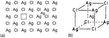
Figure 6. (a) Schematic two-dimensional illustration of a Frenkel defect in AgCl. (b) The interstitial site in three dimensions.
Download figure:
Standard image High-resolution imageIn the case of silver chloride, for instance, the formation of a 'Frenkel pair' may be written as
The symbols denote 'structure elements', in the notation introduced later by Kröger and Vink [44]. Here, □ stands for a vacant position and subscripts Ag and i for a silver site and an interstitial site, respectively, while upper indices ( and ') denote the electric charge (positive and negative) relative to the perfectly ordered crystal lattice.
Evidently, the equation describes a chemical reaction in the solid state. Rewritten in terms of 'building elements',  and |Ag|' =(□Ag' − AgAg), which may be assigned chemical potentials [45], the equation becomes
  .
.
As pointed out by Frenkel, there is an obvious equivalence to dissociation processes in gases or liquid solutions and in particular to the formation of H+ and OH− ions in liquid water.
On the basis of the formation reaction for Frenkel pairs, Frenkel was able to derive an equation that related the degree of Frenkel disorder, αFrenkel, to the standard Gibbs energy for the formation of 1 mol of (independent) Frenkel pairs, Δ G ° Frenkel. His procedure was straightforward. With αFrenkel denoting the fraction of interstitial cations or cation vacancies, referred to the total number of cations, Frenkel could easily identify the square, αFrenkel2, with the law-of-mass-action constant, KFrenkel = exp ( - Δ GFrenkel ° /RT). This led him to his famous equation
Typical values of Δ GFrenkel ° have turned out to be of the order of 100 kJ mol−1, corresponding to values of αFrenkel of about 10 - 6 at 100 °C and of about 6 × 10 - 4 at 400 °C.
Two more facts will become apparent in the next subsection:
- (i)Frenkel's result is recovered in the statistical treatment.
- (ii)Frenkel's argument is also applicable to the case of Schottky disorder, where the same equation holds after replacing αFrenkel and Δ GFrenkel ° with αSchottky and Δ GSchottky °, respectively.
6.2. Carl Wagner (1901–1977) and Walter Schottky (1886–1976): 'Theory of ordered mixed phases' (1930)
When Carl Wagner joined Max Bodenstein's institute in Berlin in 1927, he met with Wilhelm Jost who had worked with Carl Tubandt on ionic conduction and diffusion in solids. In Carl Wagner's own words1, this was the beginning of his interest in defects in ionic crystals. During his first four weeks in Berlin, he also met Walter Schottky, who gave a seminar at Fritz Haber's institute. At the end of the colloquium, Schottky was so impressed by Wagner's contributions to the discussion that he spontaneously invited him to collaborate with him and to co-author a book on thermodynamics. The famous monograph 'Thermodynamik' by Schottky et al [15] was then published in 1929. It already contained Wagner's and Schottky's ground-breaking new theory on binary ordered compounds that exhibit deviations from the ideal stoichiometric composition [16]. In particular, the book as well as their 1930 paper entitled 'Theory of ordered mixed phases' [16] included Wagner's and Schottky's rigorous treatment of point disorder in crystal lattices.
The work of Carl Wagner and Walter Schottky is, indeed, of fundamental significance for the development of Solid State Ionics, mainly for two reasons.
- (i)It provided the basis for our understanding of the equilibrium thermodynamics of point defects in ionic crystals.
- (ii)The equilibrium properties of mixed phases, and in particular their deviations from the ideal stoichiometry, were shown to depend on the chemical potentials of the components. The explanation of the phenomenon of mixed electronic and ionic conduction opened up an entire new field of electrochemistry.
In the following, these two topics will be briefly outlined, along with pertinent later work by Carl Wagner, Wilhelm Jost, Walter Schottky and others.
Figure 7 shows a photo of Carl Wagner at a later time, around 1970.
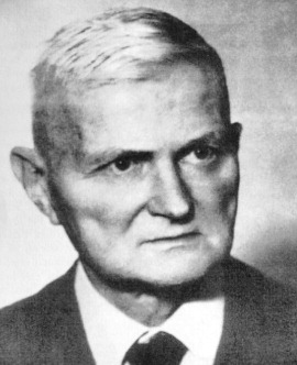
Figure 7. Carl Wagner, about 1970, with permission of Deutsche Bunsen-Gesellschaft für Physikalische Chemie.
Download figure:
Standard image High-resolution image6.3. Point defect thermodynamics in ionic crystals
In a stoichiometric binary ionic crystal of type AB, Schottky and Wagner envisaged four possible (extreme) cases of point disorder [16]. Type 1 was Frenkel disorder, with a small fraction of the cations, A+, residing at interstitial sites and an equal number of vacant sites in the regular cation sublattice. The reverse situation, with interstitial anions, B−, plus anion vacancies, constituted type 2, sometimes called anti-Frenkel disorder. A crystal of type 3 was supposed to contain no vacancies, but equal numbers of interstitial cations and interstitial anions. Finally, there were no interstitial ions in a crystal of type 4, but equal numbers of anion vacancies and cation vacancies, as sketched in figure 8.
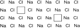
Figure 8. Schematic two-dimensional illustration of Schottky disorder in sodium chloride.
Download figure:
Standard image High-resolution imageAnti-Frenkel disorder was (correctly) supposed to be realized only in those relatively rare cases where the anions were smaller than the cations, and type 3 appeared improbable for steric reasons. On the other hand, type 4 was found to be of similar importance as type 1. It is now known as Schottky disorder [19] and is typically found in the alkali halides, cf figure 8.
We now follow Carl Wagner's and Walter Schottky's treatment in deriving the degree of Schottky disorder from the point of view of equilibrium thermodynamics. To this end, let us consider an ionic crystal AB that is made up of N cations and N anions, at ambient pressure and temperature T.
In thermal equilibrium, this crystal is supposed to contain n = n0 Schottky pairs, which contribute a (negative) amount, GSchottky (n0 ), to its Gibbs energy. The equilibrium degree of Schottky disorder, αSchottky = n0 /N , is then derived from the minimum condition
as sketched in figure 9.
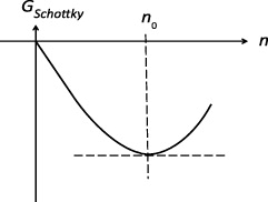
Figure 9. Sketch of the minimum condition for GSchottky (n).
Download figure:
Standard image High-resolution imageIn the expression GSchottky (n) = nΔ GSchottky ° /NA - TSconf (n), the term Δ GSchottky ° denotes the standard molar Gibbs energy of formation for (independent) Schottky pairs, NA is Avogadro's constant and Sconf (n) is the configurational entropy associated with the large number, W(n), of different possible arrangements of the 2n vacancies in the crystal lattice.
Once W(n) is formulated,  , Sconf (n) is obtained with the help of the Boltzmann equation,
  , and Stirling's approximation for factorials of large numbers. If n is much smaller than N, the required derivative, dSconf(n)/dn, takes on a particularly simple form,
  . The minimum condition then becomes
and the resulting degree of Schottky disorder is
In the case of Frenkel disorder, an analogous procedure is found to reproduce the result for αFrenkel, as given by Frenkel in 1926 [42].
In the 1930s, it was still an open question whether a given ionic crystal AB would exhibit Frenkel or Schottky disorder. In the case of AgBr, this question could be decided experimentally by Wagner and Beyer [46]. As early as in 1936 they first used a technique that was later named after Simmons and Ballufi [47], i.e. they compared the numbers of ions per elementary cell as obtained from x-ray diffraction and from density measurements. They could thus show that in AgBr only Frenkel disorder was compatible with their experimental results.
Another question concerned the alkali halides. For instance, if cation and anion were of similar size, as in KF, would the standard molar formation enthalpy be lower for Schottky or Frenkel pairs? The experimental results obtained from activation energies for ionic conduction and diffusion suggested molar formation enthalpies that were much lower than the molar lattice energies [48]. An answer to this conundrum was given by Wilhelm Jost in 1933 [49]. Jost suggested that, similar to ions in aqueous solutions, a (effectively charged) vacancy in a crystal will polarize its neighborhood, cf figure 10, and thus reduce the value of its formation enthalpy by a considerable amount.
Figure 10. Schematic view of polarization of the neighborhood of a cation vacancy.
Download figure:
Standard image High-resolution imageThe reduction of the formation enthalpy due to polarization being more pronounced for vacancies than for interstitial ions [49], Schottky correctly concluded that the close-packed alkali halide phases should all exhibit Schottky disorder [19].
Once the concept of point disorder had been introduced, ionic transport in ionic crystals became easy to visualize. On an atomic scale, the relevant processes were identified as site exchanges of mobile ions with either vacancies or vacant neighboring interstitial sites. For any of these mechanisms, the activation enthalpy for ionic conduction and diffusion must then consist of two terms, one of them, Δ Hdefect ° /2, being half the standard molar enthalpy of formation of a defect pair, and the other, Δ m H, being the (molar) 'migration enthalpy' required for the site-exchange itself. In thermal equilibrium, this would result in a conductivity which, in a plot of  versus 1/T , was represented by a straight line with slope - (1/R)(Δ Hdefect ° /2 + Δ m H). In the schematic plot of figure 11, this line is seen at sufficiently high temperatures, where thermal equilibrium is attained within the experimentally available period of time.
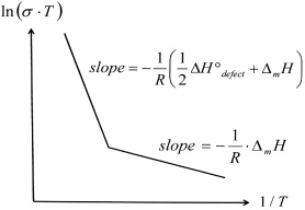
Figure 11. Schematic view of temperature-dependent ionic conductivity via point defects.
Download figure:
Standard image High-resolution imageIt had, however, also become obvious that thermal equilibrium was not attained at lower temperatures, where the slope of  versus 1/T was found to be only - Δ m H/R [48]. This suggested that the actual number density of defect pairs had to be regarded as 'frozen in' from an equilibrium state at higher temperature.
For the case of Schottky disorder, it was soon realized that this effect had to be expected, since temperature-dependent adjustments of the equilibrium number densities of vacancies would necessitate many ions being transported throughout the sample volume. On the basis of a rough estimate, Wilhelm Jost was able to show that the required time would clearly exceed the time for which an experimenter might be able (or be willing) to wait [48].
Another possibility for the actual degree of disorder being higher than expected, and constant at low temperatures, was seen to originate from the presence of heterovalent ions. Consider, for instance, an ionic crystal AB, in which some of the monovalent cations on regular lattice sites are replaced by divalent impurity ions such as Ca2+ or Mg2+. Clearly, this must be accompanied by an identical number of cation vacancies, for reasons of charge neutrality, and can thus explain the low-temperature branch in the plot of figure 11.
More importantly, an intentional replacement of a considerable fraction of the tetravalent cations in ceramic materials such as ceria and zirconia by heterovalent cations such as La3+ or Y3+ must imply the creation of a substantial number of vacancies in the oxygen sublattice. As a result, one obtains a solid electrolyte that exhibits excellent oxygen-ion conduction, in particular at elevated temperatures. This mechanism was already exploited by Walther Nernst in his Nernst mass, but identified only much later, in 1943, by Carl Wagner [28].
6.4. Deviations from the ideal stoichiometry; mixed ionic and electronic conduction
In their thermodynamic treatment of ordered mixed phases, Wagner and Schottky were led by the insight that in a system (A, B) the equilibrium properties of each phase are only determined if, besides temperature and pressure, the chemical potentials of the components are also fixed [16]. An example is given in figure 12.
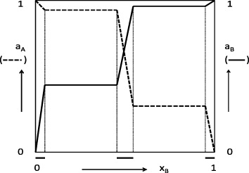
Figure 12. Schematic view of dependence of activities of two components on composition, if homogeneous phases exist in the regimes marked by bars on the molar-fraction axis.
Download figure:
Standard image High-resolution imageIn this case, some B is soluble in solid A and vice versa, and there is a homogeneous binary mixed phase with a finite width around xA = xB = 0.5. In figure 12, the composition regimes of the three homogeneous solid phases are separated by two broad two-phase fields. The figure shows how the composition in each homogeneous phase is defined by the activities, and thus by the chemical potentials, of its components.
In their statistical-mechanical treatment, Wagner and Schottky considered especially the defect structures of intermetallics such as CuZn. The lattice defects were shown to be decisive for the widths of the one-phase fields and, conversely, experimental data for field widths could be used to determine the concentrations of the lattice defects [16].
In his subsequent 1933 paper [18], Carl Wagner addressed the defect properties of polar compounds that exhibit finite field widths in their respective phase diagrams. He recognized that in metal oxides such as ZnO an excess of metal implied the existence of mobile electrons that caused electronic conduction, while a deficit of metal as in Cu2O or NiO caused electronic conduction due to holes [18]. By coincidence, the concept of electron holes had just before been introduced by Rudolf Peierls [50] and Werner Heisenberg [51].
In particular, Carl Wagner pointed out that in ionic compounds such as Ag2+δS deviations from the exact stoichiometry,  , were indicative of the presence of both ionic and electronic defects, the value of δ being connected with the molar fractions of the electrons and holes via δ = xe - xh. Also, assuming ideal solution behavior for electronic defects, a law-of-mass-action equilibrium condition, xe xh = const, had to be fulfilled for the formation reaction of electrons and holes.
For mixed ionic/electronic conductors not featuring the exceptional property of structural disorder (now disregarding α-Ag2+δS, see below) any deviation from the exact stoichiometric composition necessarily implied that not only the numbers of electrons and holes but also the numbers of effectively positive and negative lattice defects had to differ from each other. In the case of Frenkel disorder, for instance, the equation 0 = μi + μV would have to contain different molar fractions, xi and xV, the indices i and V denoting the building elements 'interstitial site occupied' and 'regular site vacated', respectively. Once the chemical potentials were expressed by xi and xV, a law-of-mass-action equilibrium condition was obtained for the product, xi xV, while the difference, xi - xV, was determined by δ.
Likewise, equilibrium conditions could also be formulated for incorporation reactions. As might have been expected, the molar fractions of all ionic and electronic defects finally turned out to be well defined as soon as (besides temperature and total pressure) the chemical potential of one component was fixed, the other being given by the Gibbs–Duhem equation.
In the mid-1950s, Brouwer (The Netherlands) [52] as well as Kröger and Vink (The Netherlands) [53] used Carl Wagner's early views to derive a large number of 'defect diagrams', also called Brouwer or Kröger–Vink diagrams, such as the one of figure 13.
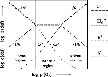
Figure 13. Brouwer diagram for defects in an oxide, M2O1+δ, featuring anti-Frenkel disorder. In the definition of the ordinate, x (def) and z (def) denote molar fractions and charge numbers. The slopes result from the equations for the laws of mass action and for electroneutrality. Of course, there should be smooth transitions at the crossing points [54].
Download figure:
Standard image High-resolution imageThe example considered in figure 13 is a ceramic material, M2O1+δ, featuring anti-Frenkel disorder in the oxygen lattice [54]. Here, δ is the difference between the molar fractions of interstitial oxygen ions and oxygen vacancies, and also (apart from a factor of two) the difference between the molar fractions of holes and electrons. The equations required for the construction of the Brouwer diagram include electroneutrality as well as the laws of mass action for anti-Frenkel disorder, for the formation of electrons and holes, and for the incorporation of oxygen from the outside. Note that the partial pressure of oxygen, p(O2), which is proportional to the oxygen activity, serves as a measure for the chemical potential of oxygen.
In retrospect, it can be stated that our understanding of mixed ionic and electronic conduction, now often called MIEC2, is indeed based on Carl Wagner's pioneering work.
At this point, we resume reporting on Carl Wagner's studies of silver sulfide, which was his favorite model system3. Earlier investigations into the electric conductivity of silver sulfide, by C Tubandt and co-workers, had not only provided answers, but also questions. Firstly, the material was apparently a mixed ionic and electronic conductor (MIEC), both above and below its β to α phase transition at about 450 K (depending on δ, cf figure 14). However, this result came along with a big puzzle [31, 57]. Faraday's first law seemed to be invalidated since, in a cell that used a layer of α-AgI in contact with silver sulfide for blocking out the electronic conductivity, the transport number of the silver ions was unexpectedly found to be one. Secondly, it was observed that the electrical conductivity of silver sulfide changed reversibly with sulfur pressure [31, 58]. Why was this so?

Figure 14. Schematic view of part of the Ag–S phase diagram in the α/β transition region after [56].
Download figure:
Standard image High-resolution imageCarl Wagner could answer both questions by regarding α- and β-Ag2S as mixed phases with finite field widths, Ag2+δS. The first puzzle was then solved by allowing for the development of a gradient of the chemical potential of silver inside silver sulfide, with internal fluxes of ions and electrons resulting from it [56, 59]. Tubandt's and Reinhold's second observation [31, 58] was, indeed, in perfect agreement with the expectations according to figure 12. Evidently, the chemical potential of sulfur in silver sulfide varied with sulfur pressure, entailing the corresponding variations of composition, defect structure and transport properties.
What was still lacking in the 1930s, was an experimental technique that could be used in order to determine the relationship between tiny deviations from the exact stoichiometric composition, δ, on the one hand and the activities (or chemical potentials) of the components on the other, as in figure 12. Such a technique, with the potential of making visible variations of δ on the order of 10 - 9, was invented by Carl Wagner in 1953 [60]. He called it 'coulometric titration', see below, and showed how to use it for the construction of detailed phase diagrams.
In the schematic plot of figure 14, for instance, the width of the β-Ag2S phase field was thus found to be less than 10 - 5, while that of α-Ag2S is about 2 × 10 - 3. For clarity, the figure does not include the (nearly vertical) iso-activity lines for the components within the two one-phase fields, which were determined later, with the help of Wagner's titration technique, see the excellent review on Ag2S written in 1980 by Schmalzried [61].
In 1953, Carl Wagner employed the following galvanic cell for his coulometric-titration experiments on silver sulfide:
Here, α-AgI was again used to block out the passage of electrons. The relative chemical potential of silver in Ag2+δS was obtained by the measurement of the e.m.f. of the cell, E, according to

Applying an outer voltage to the cell and measuring the product of electric current and time, it was now easy to change the silver content in the sulfide at will, by 'titration' in very small steps of Δ δ ≈ 10 - 9. Compositions could thus be related to silver activities at any chosen temperature, and the data could then be used, e.g., for constructing iso-activity lines in plots like figure 14.
Having called α-AgI the archetypal solid electrolyte, we may likewise consider α-Ag2+δS the archetypal MIEC.
In α-Ag2+δS, the sulfur-ion sublattice is bcc, just like the iodide sublattice in α-AgI [62, 63]. As in α-AgI, the silver ions are structurally disordered, and their motion may be regarded as liquid-like. Their coefficient of self-diffusion is found to be similar to α-AgI [64, 65] and, consequently, the same holds true for their partial conductivity [32, 66]. Unlike α-AgI, however, α-Ag2+δS exhibits an electronic conductivity that surpasses the ionic one by two orders of magnitude. Its value depends on composition and slightly increases as a function of inverse temperature, see figure 15 [67].
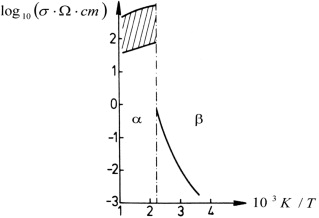
Figure 15. Conductivity versus inverse temperature for Ag2S in the α/β transition region; according to [67].
Download figure:
Standard image High-resolution imageOn the other hand, the silver ions are not structurally disordered in the low-temperature β-phase. In β-Ag2S, both ionic and electronic conductivity are much lower than in α-Ag2+δS. The electronic conductivity of β-Ag2S is found to increase with increasing temperature, suggesting a polaronic transport mechanism [67].
It is worth mentioning that, quite generally, partial ionic/electronic conductivities of mixed ionic electronic conductors are measured by blocking out the electronic/ionic component. This is the principle of the so-called Hebb–Wagner polarization technique [68, 69]. For instance, a setup suitable for measuring the ionic conductivity of silver sulfide is Ag|α-AgI|Ag2+δS|α-AgI|Ag.
This section would remain incomplete, if no reference was made to the modest integrity of Carl Wagner's personality. In his own words, 'modesty makes you feel free'.
7. AgI-type solid electrolytes
7.1. Ionic conductivities
The two panels of figure 16 are Arrhenius plots of the ionic conductivities of those AgI-type solid electrolytes that had been discovered by Carl Tubandt and his co-workers [20, 30]. These materials were, therefore, known in the 1930s, when the study of solid ion conductors developed into a field of renewed interest in Europe.
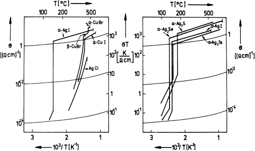
Figure 16. Ionic conductivities of AgI-type solid electrolytes. Left-hand panel: highly cation-conducting silver and cuprous halide phases. Right-hand panel: highly cation-conducting silver chalcogenide phases (plus AgI for comparison). From [70], with permission of Pergamon Press.
Download figure:
Standard image High-resolution imageLike α-AgI itself, all members of this group are characterized by cationic conductivities in excess of 1 Ω−1 cm−1. In the 1930s, it became evident that there were two prerequisites for such easy ion transport, namely (i) structural disorder of the cation sublattices and (ii) small migration enthalpies [48]. More explicitly, the features that these materials have in common were found to be the following:
- (i)The cations are structurally disordered in the sense that the number of voids provided for them by the anion lattice by far exceeds their own number, and that there is no optimum distribution of them. Typically, a cation can always find vacant voids in its immediate neighborhood.
- (ii)The anions are so arranged that the local potentials felt by the cations are rather flat along pathways that interconnect neighboring voids.
Over time, it became apparent that the highly ion-conducting phases of figure 16 share the above properties with a number of other AgI-type solid electrolytes. The ionic conductivities of some of them, which have more complex chemical compositions and were discovered later, are shown in figure 17.
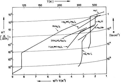
Figure 17. Ionic conductivities of several AgI-type solid electrolytes (plus AgI for comparison). From [70], with the permission of Pergamon Press.
Download figure:
Standard image High-resolution imageIn the highly conducting silver and cuprous halides, the transport numbers of the electrons were shown to be much smaller than one. In 1954, Jost and Weiss [71] reported a value of less than 10 - 7 for α-AgI, and in 1957 Wagner and Wagner [72] found values of about 10 - 5 and 10 - 4 for β-CuBr and α-CuI, respectively.
On the other hand, electronic conduction predominates in the chalcogenides.
The solid electrolytes referred to in figure 17 are all silver ion conductors with negligible electronic transport numbers. They were derived from AgI by partial substitution of the silver or the iodide ions, or even both, by different kinds of ions. Thus new compounds were obtained, which in some cases exhibit unusually high ionic conductivities even at room temperature and below.
As the first example of this group of materials, α-Ag2HgI4 was described by Ketelaar (The Netherlands) [73] in 1934, the transport numbers being roughly 0.94 for Ag+ and 0.06 for Hg2+. In 1961, Reuter and Hardel (Germany) [74] reported ionic conductivity data of Ag3SI in its α- and β-phases. A further big step forward was made in 1966 and 1967, when Bradley and Greene (UK) [75, 76] and Owens and Argue (USA) [77] independently discovered a group of solid electrolytes of composition MAg4I5, where M represented Rb, K or NH4. At room temperature, these compounds exhibited the largest known solid state ionic conductivities [75–77], e.g. 0.27 Ω−1 cm−1 in the case of RbAg4I5 [78]. The other silver-ion conductors included in figure 17 were found a few years later by Japanese [79, 80] and American [81–83] scientists.
7.2. Structures
Besides α-AgI, the phases α-CuBr, α-Ag3SI, α-Ag2S and α-Ag2Se also have bcc anion structures, see below. The number of cations per bcc unit cell is two in α-AgI and α-CuBr, three in α-Ag3SI and four in α-Ag2S and α-Ag2Se. The following brief overview begins with α-AgI.
In the mid-1970s, shortly before Cava et al [35] published their single-crystal results, powder neutron-diffraction experiments on α-AgI had independently been performed by Bührer and Hälg (Switzerland) [84] and by Wright and Fender (UK) [85], already providing clear evidence that the silver ions spent most of their time in the tetrahedral voids of the bcc iodide lattice.
In 1975, Bührer and Brüesch (Switzerland) [86] were able to explain why the reorganization of the iodide ions at the transition from the wurtzite-type β-phase to the bcc α-phase of AgI required only a small amount of energy. They showed that this was due to the existence of a very low-lying (2 meV) phonon branch in β-AgI, observed at the zone center. Long-wavelength phonons of this mode can provide the displacements of the iodide ions necessary for their rearrangement at the phase transition as illustrated in figure 18.
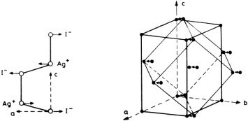
Figure 18. Left-hand panel: ionic displacements associated with low-energy, long-wavelength phonons in β-AgI. Right-hand panel: this phonon mode supports the rearrangement of the anions at the transition from β-AgI to α-AgI [86].
Download figure:
Standard image High-resolution imageIn 1952, Krug and Sieg in Germany [87] and Hoshino in Japan [88] independently ascertained that α-CuBr was isostructural with α-AgI, with regard to both the bcc anion lattice and the disorder of the cations.
As expected, the silver ions were found to be structurally disordered in the bcc phases α-Ag2S and α-Ag2Se as well, possibly with slight preferences for the tetrahedral voids in α-Ag2Se, as suggested by Rahlfs in 1936 [62], and for the octahedral voids in α-Ag2S, as proposed by Rickert in 1960 [89].
The structure of α-Ag3SI was established by Reuter and Hardel in 1965 [90]. In the case of this high-temperature phase, the sulfide and iodide ions were shown to be statistically distributed over the sites of a bcc anion lattice, while the silver ions were again structurally disordered.
On the other hand, β-Ag3SI as well as Ag3SBr exhibited ordered anion structures [90]. The bcc anion lattices could now be regarded as being composed of interpenetrating simple cubic sublattices, with the halide and sulfide ions residing at the 0, 0, 0 and 1/2, 1/2, 1/2 sites, respectively. The number of silver ions and the number of faces of halide cubes being identical, it was concluded that the Ag+ ions were most of the time confined to the faces of those cubes, implying that, in the strict sense of the word, the cations were no longer structurally disordered.
A nuclear density map constructed for β-Ag3SI from neutron diffraction data in 1986 [91] provided evidence for a broad distribution of the silver probability density on each face center of the iodide cubes, the root-mean-square displacement being as large as 60 pm. Three years later, a broad maximum in the 295 K conductivity spectrum, extending from about 25 GHz to more than 1 THz, could be attributed to localized diffusive motion of the silver ions on the cube faces [92]. Indeed, the observed unusual feature was well reproduced with the help of a Langevin equation in two dimensions, with a typical liquid-state value for the coefficient of self-diffusion and a root-mean-square displacement of about 60 pm.
By contrast with α-AgI and α-CuBr, the high-temperature phase of cuprous iodide, α-CuI, was found to have a face-centered cubic (fcc) anion lattice [87]. This was not unexpected in view of the ratios of the cationic to anionic radii of these three compounds, since the voids provided by an fcc anion lattice are smaller than those in a bcc structure. In the fcc lattice, the optimum diffusion pathways for the mobile cations are along alternating unlike voids: tetrahedral, octahedral, tetrahedral, etc.
A close-packed structure was also assigned to the anions in β-CuBr [87, 88]. This time, however, the structure is hexagonal, and the most probable diffusion paths for the cations are those that interconnect face-sharing octahedra [93].
In α-Ag2HgI4, first analyzed by Ketelaar in 1934 [94], the three cations statistically occupy the four zincblende-type voids in the fcc unit cell. On average, one of them thus remains unoccupied. For this reason, very high ionic conductivities were already predicted [94] prior to their measurement.
The structure of α-RbAg4I5 was first determined in 1967, independently by Bradley and Greene in the UK [95] and by Geller in the USA [96]. The cubic unit cell contains 24 Ag1 voids and 24 Ag2 voids for 16 silver ions, forming channel-like diffusion paths that traverse the crystal in the 〈100〉 directions in a zigzag fashion, cf figure 19.
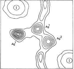
Figure 19. Partial Fourier density map of the silver ions in α-RbAg4I5 at z = 0, at room temperature [97]. None of the silver sites is exactly centered in the z = 0 plane. By courtesy of W F Kuhs and G Heger.
Download figure:
Standard image High-resolution imageThe Fourier density map of figure 19 was constructed by Kuhs and Heger in 1981 [97], on the basis of neutron-diffraction data obtained at the Institut Laue-Langevin, Grenoble, France. It shows a section of one out of six channels per unit cell, two of them extending in each Cartesian direction. The map also shows how orthogonal channels are interconnected by pairs of Ag1 voids, allowing the silver ions to change from one channel to another.
RbAg4I5 undergoes phase transitions at 209 K and 122 K [99]. The one at 122 K is of first order and involves a sudden decrease in conductivity, cf figure 17. The structure of the low-temperature γ-phase was unknown until 2006. In this phase, the existence of locally mobile silver ions had been predicted on the basis of high-frequency conductivity measurements. This was then verified by a structural refinement of x-ray diffraction data taken at the synchrotron in Grenoble [98]. It was thus shown that about 56% of the silver ions are contained within structural pockets, where they are locally mobile, see figure 20, while those that traverse the crystal along pathways for translational motion do so via a vacancy mechanism.

Figure 20. Perspective view of the crystal structure of γ-RbAg4I5. White balls mark possible silver-ion positions contained in structural pockets between distorted RbI6 octahedra [98]. These 'partially occupied positions' should, however, not be taken too literally, but rather as an indication of a novel 'local' kind of disorder.
Download figure:
Standard image High-resolution image8. An evolving scheme of materials science
As discussed in the previous sections, disorder is of the essence of Solid State Ionics. Different levels of disorder are highlighted in figure 21. In this 'evolving scheme of materials science', perfectly ordered crystals are placed at level one. At this level, there is no possibility for the ions to leave their sites. Historically, the decisive step forward was made when site disorder was discovered and point-defect thermodynamics were developed. At this stage, level two, ionic transport is accomplished by mobile point defects. In fact, modern materials science and engineering largely build on the concept of level two.
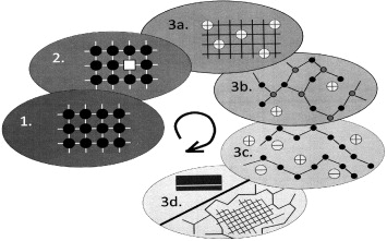
Figure 21. An evolving scheme of materials science: 1—ideally ordered crystals; 2—point disorder in crystals; 3a—crystals with structural disorder; 3b—ion-conducting glasses; 3c—polymer electrolytes; 3d—nanosized systems such as nano-composites and thin films.
Download figure:
Standard image High-resolution imageDramatic changes are encountered as we move on to structurally disordered materials, that is, from level two to level three. At this level, ionic transport can no longer be described in terms of individual defects that move in a static energy landscape. Instead, we are facing a challengingly complicated many-particle problem, with the mobile ions interacting with each other and with their surrounding matrix. This applies to structurally disordered ionic crystals (level 3a), to ion-conducting glasses (level 3b), to polymer electrolytes (level 3c) and to nanosized systems (level 3d).
The evolving scheme of figure 21 is remarkable for different reasons. It records a historical development leading to new classes of increasingly complex ion-conducting materials. The attainment of each new level meant new scientific challenges regarding the investigation of the structures and ion dynamics of its members. At the same time, increasingly favorable possibilities for applications in devices were offered by each new class of materials.
In the course of the scientific and technological advancement along the evolving scheme, essential steps of progress have been taken in Europe. Some of these will be outlined in the following subsections, along with a sketch of the development of our understanding of the ionic materials of figure 21.
In the first place, however, let us briefly mention those instant 'eye openers' that are now, in retrospect, well remembered for having caused a new awareness and visibility of Solid State Ionics in both academia and the public.
The discoveries of the structurally disordered crystalline fast-ion conductors (level 3a) rubidium silver iodide [75–77] and sodium-beta-alumina [100], in the late 1960s, were indeed the first spectacular milestones in the field of Solid State Ionics attained during the past half century. The advent of RbAg4I5, for instance, created hopeful prospects for compact batteries [101, 102] that might operate at room temperature, in satellites and cardiac pacemakers, while Na-β-alumina, discovered by Yao and Kummer in the USA [100], was viewed as the solid sodium-ion conductor par excellence, to be employed in sodium/sulfur batteries [103, 104], which might be used for automotive propulsion.
In the late 1970s, glassy and polymeric electrolytes appeared on the stage of Solid State Ionics, offering new possibilities that had been unthought-of before. It was then realized that huge conductivity ranges were spanned by ion-conducting glasses (level 3b) [105–107] and that the mobile ions in them had to be regarded as dynamically decoupled from the rigid matrix [107]. As in crystalline electrolytes, this resulted in conductivities that were Arrhenius-activated. These could attain values as high as 0.03 Ω−1 cm−1 at room temperature, with activation energies as low as 20 kJ mol−1 [108], see the pertinent subsection below.
In comparison to glasses, polymer electrolytes (level 3c) turned out to exhibit lower conductivities, but thin-film cell configurations could largely compensate for those lower values [109].
Unlike ion-conducting glasses, polymer electrolytes, usually considered above their glass transition temperatures [110], proved to be dynamically coupled systems [107], with virtually identical time constants characterizing the decay of electric fields and mechanical deformations in them, due to ionic motion and segmental motion, respectively. In Arrhenius diagrams, lines showing a pronounced downward bend were obtained for ionic conductivities as well as inverse viscosities [107, 111]. These lines have always been found to be very similar in shape and have often been described by the empirical Vogel–Tammann–Fulcher (VTF) relation [112–114], see again the pertinent subsection.
In the 1980s, yet another type of structural disorder in solids came into view [115, 116], with substantial consequences for the defect thermodynamics and the dynamics of mobile ions (and electrons). At that time it was realized how the properties of nanosized systems such as nano-composites and very thin films (level 3d) were governed by their inner and outer surfaces and how this resulted in transport coefficients that were often drastically different from the polycrystalline materials [116]. A new field of research was thus born, namely nanoionics [117, 118]. This will be touched upon in the last of the following subsections.
Since the early 1970s, the rapid advancement along the evolving scheme, as sketched above, has been accompanied by international meetings and conferences. The first few of them were entitled 'Fast Ion Transport in Solids', 'Superionic Conductors' and 'Solid Electrolytes', while the biennial ones held from 1983 onward have been announced as 'International Conferences on Solid State Ionics'. The International Society of Solid State Ionics was founded at one of them, held at Garmisch-Partenkirchen, Germany, in 1987.
Early on, these meetings and conferences documented a widening of the range of topics, with an increasing trend to include not only basic science, but also applications and devices. In the years and decades to follow, the effort to find suitable materials and techniques for the storage and conversion of energy, for sensing and other applications has become ever more pronounced.
Current interest in fuel cells and batteries for the future focuses mostly on crystalline lithium-ion, oxide-ion and proton conductors as electrolytes, as well as ion-conducting glasses and thin-film polymers. In either case, MIECs are most promising as reversible electrode materials. The final section of this review is dedicated to such ionic and mixed conductors and to their applications in devices that pursue the aim of environmental sustainability.
At this point, let us resume our brief outline of the levels of disorder as presented in figure 21.
8.1. Crystalline electrolytes: from isolated point defects to structural disorder
When Frenkel, Wagner and Schottky introduced the concept of point defects, these were viewed as in the sketch of level two in figure 21, i.e. as non-interacting individual charge carriers that performed perfectly random walks throughout the crystal volume. The validity of this view could, however, be checked only much later, by the combined application of frequency-dependent experiments and linear response theory.
According to linear response theory [119], the frequency-dependent conductivity of a system of identical mobile charge carriers is proportional to the Fourier transform of their velocity correlation function,  . Suppose the charge carriers are random walkers. As random walkers have no memory, the self terms,
  , consist only of a delta-type peak at t = 0, reflecting the self-correlation during a hop. Also, random walkers do not know of each other, which results in cross terms,
  with
with  , that vanish at all times. As the Fourier transform of a delta function at t = 0 is a constant, a system of charged random walkers will result in a conductivity that does not depend on frequency.
In fact, the ionic conductivity of crystalline AgBr, at 200 °C, has been found to be frequency-independent up to the microwave regime, thus conforming with the expectations for a system of random walkers [120]. According to Corish and Mulcahy (UK) [121] the silver ions in AgBr are supposed to move via the collinear interstitialcy mechanism, which means that an interstitial silver ion can replace a silver ion on a regular lattice site by shifting it forward into another interstitial site. In the case of AgBr, the 'random walkers' may, therefore, be identified with moving interstitialcies.
Another clear-cut example is strontium chloride, SrCl2, at 1050 K, where anion vacancies have been shown to play the role of random walkers [122]. Like PbF2, SrCl2 crystallizes in the fluorite structure, cf figure 22, and displays a Faraday transition into its highly anion-conducting state. At 1050 K, Dickens et al (UK) [122] have taken incoherent quasi-elastic neutron-scattering spectra of a single crystal of SrCl2 in order to study the hopping motion of the chloride ions.
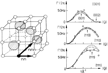
Figure 22. Left-hand panel: the fluorite structure; nearest-neighbor (nn) and next-nearest-neighbor (nnn) hopping vectors. Right-hand panel: experimental and calculated widths of the incoherent scattering function,  , for SrCl2 at 1050 K, with
  in three different crystallographic directions [122].
Download figure:
Standard image High-resolution imageThe experimental spectra could be directly compared with different model spectra, by using the treatment pioneered by Chudley and Elliott (UK) [123]. The authors were thus able to rule out ionic hopping via interstitial sites. In figure 22, the broken and full curves are best fits for ionic hopping via ordinary lattice sites, i.e. via nearest-neighbor sites and via nearest-neighbor plus next-nearest-neighbor sites, respectively. The chain curves, however, result from an even more realistic model. In this model, the chloride ions perform their jump diffusion by means of 'encounters' with vacancies, which are themselves supposed to be random walkers [124].
Many more examples have been given for transport mechanisms via point defects in ionic crystals, for instance, in 1957 by Lidiard (UK) [125] and later in [126, 127]. This included the effects of defect association, first discussed by Teltow [128] and Lidiard [129]. Atomistic defect calculations as first introduced by Mott and Littleton (UK) in 1938 [130] were subsequently developed further and successfully employed in the HADES program (UK) [131], the acronym standing for Harwell Automatic Defect Evaluation System. For some of the major results see, for instance, the book by Hayes and Stoneham (UK) [132].
It is now well known that the random motion of defects in fast ion conductors must be considered the exception rather than the rule. This is most obviously seen in the characteristic and ubiquitous frequency dependence that is normally displayed by their ionic conductivities. The example shown in the left-hand panel of figure 23 [133, 134] is representative, and others will be given in the next subsections.
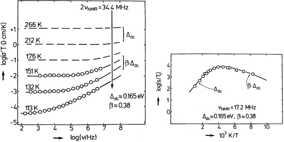
Figure 23. Left-hand panel: dynamic conductivity of Na-β-alumina [133, 134]. Right-hand panel: sodium spin–lattice relaxation rate of Na-β-alumina at 17.2 MHz [135].
Download figure:
Standard image High-resolution imageIn 1977, Grant et al (UK) [133] first reported on the frequency-dependent conductivity of a single-crystalline solid electrolyte, which was Na-β-alumina, and more conductivity data of this system were presented later by Almond et al (UK) [134]. Here we recall that the famous sodium-ion conductor Na-β-alumina had been discovered by Kummer et al (USA) [100, 103], who had announced the development of a sodium/sulfur battery. In that battery, solid Na-β-alumina separated the electrodes, which consisted of molten sodium and molten sulfur.
In the two panels of figure 23, a comparison is given of the frequency-dependent ionic conductivity of Na-β-alumina at different temperatures [133, 134] and its temperature-dependent sodium spin–lattice relaxation rate at fixed frequency [135].
For a better appreciation of the meaning of the figure, it is helpful to consider some aspects relating to the structure of Na-β-alumina and its conduction mechanism.
In Na-β-alumina, of composition Na1+2xAl11O17+x with 2x ≈ 0.33, sodium ions are highly mobile in conduction planes that are sandwiched between symmetrically arranged spinel blocks [136–139]. Their mobility is essentially due to the 2x 'excess' Na+ ions per formula unit. Without them, the sodium ions would occupy every second site ('Beavers–Ross' sites) on six-membered rings that form a honeycomb lattice. In the presence of the excess Na+ ions, however, only two out of the three Beavers–Ross sites on a ring are found to be occupied by Na+ ions, while the third Na+ ion pairs up with an excess sodium ion to form a 'split interstitialcy' located on either side of the third Beavers–Ross site, these sites being called 'mid-oxygen'. The 'interstitialcy pair' then migrates via an exchange-of-partners mechanism [137–139]. In view of their arrangement and dynamics, the sodium ions in Na-β-alumina must, indeed, be considered structurally disordered (level 3a).
In Na-β-alumina, the high number density of mobile charge carriers implies that the Coulomb interactions between them can no longer be ignored (as in level-two materials), resulting in non-random sequences of their hopping motion. As already pointed out in [133] and later by Funke (Germany) [140], this phenomenon bears some similarity to the Debye–Falkenhagen effect in dilute strong liquid electrolytes [141], but is much more pronounced.
In a dilute strong liquid electrolyte, a small dispersion of the conductivity is expected, for the following reason [141]. Any displacement of an ion implies that the ion no longer resides at the center of its ion cloud [142, 143]. As a consequence, relaxation sets in, with the ion moving backward and/or the cloud rearranging.
In a disordered solid electrolyte, the ion cloud is formed by the other mobile ions. Relaxation after a hop is either on the single-particle route, with the ion hopping backward, or on the many-particle route, with the cloud rearranging. The ratio of Coulomb energy by thermal energy is now considerably larger than in a dilute liquid electrolyte, due to much larger number densities of mobile ions and (in some cases) to lower temperatures. Therefore, the effect is much more pronounced, the frequency dependence of the conductivity reflecting frequent forward–backward hopping sequences of the mobile ions.
This frequency dependence is seen in the left-hand panel of figure 23. As already noted in [133] and also in later papers authored by Almond, West and co-workers (UK) [134, 144], it is nicely fitted by the power-law description suggested earlier by Jonscher (UK) [145, 146], i.e. by

where p = 1 - β, cf figure 23, is an empirical exponent. The angular frequency that marks the onset of the dispersion, ω0, corresponds to the time interval (after a hop), t0 = 1/ω0, at which the correlated backward hopping ends and random macroscopic diffusion sets in.
As long as the conduction mechanism does not change, the onset angular frequency (which has to be interpreted as the rate of random hops) must be proportional to the coefficient of self-diffusion, ω0 ∝ D ∝ Tσ (0). This is known as Summerfield scaling [147]. As a consequence, ω0 and Tσ (0) have the same activation energy, Δ dc.
For a discussion of spin–lattice relaxation rates, 1/T1, cf the right-hand panel of figure 23 and also figure 24, it is useful to consider not only the onset (angular) frequencies at given temperatures but also the inverse onset temperatures at given frequencies, 1/T0 (ν ). In the left-hand panel of figure 23, for instance, the onset temperature at 34.4 MHz may be estimated by following the vertical arrow and checking for the transition from the dc activation energy, Δ dc, to the formal activation energy in the dispersive regime, which is β Δ dc.
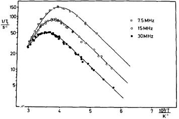
Figure 24. 1H spin–lattice relaxation rates of the hydrogen intercalation bronze H2MoO3, according to [148], by courtesy of W Müller-Warmuth.
Download figure:
Standard image High-resolution imageThe spin–lattice relaxation rate, 1/T1, is expected to attain its maximum, when (roughly) twice the Larmor angular frequency coincides with the rate of random hops, 4π νNMR = ω0. This condition, 2νNMR = ν0, is fulfilled at 1/T = 1/T0 (2νNMR ), and the rate maximum in figure 23 is indeed observed close to this value on the inverse-temperature scale. From the experimental data of the figure, it is also found that the slopes of  versus K/T are about Δ dc /kB and - β Δ dc /kB at high and low temperatures, respectively. This obviously corresponds to the values of Δ dc and β Δ dc that are encountered along the vertical line in the left-hand panel.
A more quantitative discussion can be given on the basis of 1H spin–lattice relaxation rates measured on a hydrogen intercalation bronze by Ritter et al (Germany) [148], since in this case data have been taken as a function of both temperature and frequency, see figure 24. When compared with the predictions of Bloembergen–Purcell–Pound theory [149], these data show two anomalies. In the first place, the maxima are clearly asymmetric and are thus similar to the example of figure 23. Second, the low-temperature rates show a frequency dependence which is less pronounced than the expected 1/νNMR2 behavior. Both features are easily explained in terms of a partial hydrogen conductivity that follows the 'Jonscher law'. The argument is as follows.
As spin–lattice relaxation rates and ionic conductivities can be well expressed in terms of one real function of time4, conductivity spectra of the Jonscher type may be transformed into rates, 1/T1, with the following results:
- 1.The rate, 1/T1, attains its maximum roughly at the inverse onset temperature, which is1/T0 (2νNMR ).
- 2.If 1/T is well below this value, 1/T1 will be independent of νNMR, varying with 1/T as exp (Δ dc /kB T).
- 3.If 1/T is well above 1/T0, 1/T1 will vary with νNMR as νNMR - (1+β ) and with 1/T as exp ( - β Δ dc /kB T).
In the data of figure 24, all these expectations are indeed nicely fulfilled, with p = 1 - β ≈ 0.8.
The characteristic fingerprints of σ (T,ν ) and 1/T1 (T,ν ) have been detected in many other materials as well, the only caveat (see later) being that the 'Jonscher law' is not exact, but rather a useful approximation.
So far, the purpose of this subsection has been to emphasize that, in crystalline electrolytes, an increasing degree of disorder implies increasing relevance of interactions between the mobile charge carriers, thereby drastically affecting the ion dynamics.
Additional huge effects on the ion-transport properties have been encountered in structurally disordered mixed-cation conductors. This is probably best exemplified by the Na–Li, Na–K and Na–Ag β-aluminas, which have been studied by Ingram and his co-workers (UK) [139, 150–152]. In these mixed-cation systems, the dc ('direct current') ionic conductivities were found to be lower than those of the single-cation end members by up to five orders of magnitude. Remarkably, a unique explanation could be given in terms of preferences of particular cations for particular sites. For instance, the preference of potassium ions for Beavers–Ross sites made it virtually impossible for sodium ions to displace them. Later on, these ideas of site preference and mismatch could be incorporated directly into the modeling of the mixed-alkali effect in glass, see the following subsection.
8.2. Ion-conducting glasses
New advantages and new challenges came into view, when, essentially in Europe, the Solid State Ionics community started to consider not only crystalline, but also glassy electrolytes [153–158], as represented at level 3b of figure 21.
Obviously, the advantages of ion-conducting glasses included their physical isotropy, their continuously variable composition, their good workability and the absence of grain boundaries [159]. Consequently, ion-conducting glasses were soon recognized as being well suited for a wide range of electrical and electrochemical applications.
On the other hand, the lack of long-range order made the structures and dynamics of vitreous electrolytes look extremely complicated. Evidently, at least two kinds of interaction had to be taken into account, i.e. the one between the disordered network structure and the mobile ions and, very important as well, the long-range Coulomb forces between those ions. The resulting basic challenge has been summarized in one sentence [160]: Where are the ions, how did they get there, and where do they go next?
Historically, the existence of ionic conductivity in glass was first proved in 1884, when the German physicist Emil Warburg verified Faraday's laws for the transfer of sodium through a glass membrane placed between two amalgams and could thus ascertain that the sodium transport number was one [161, 162]. Note that the unipolar conductivity of glass is important from both practical and theoretical points of view. From the practical point of view, the unit transport number in glass relates directly to the applicability of glasses in devices, for instance, of Li+-ion-conducting glasses in lithium batteries.
In the 1970s and 1980s, the recent discoveries in the field of crystalline fast ion conductors, notably of RbAg4I5 and the beta aluminas, led to an explosion of interest in the existence of possible glassy alternatives, see e.g. Kunze (Germany) [163] and Chiodelli et al (Italy) [164]. Many AgI-containing glasses were synthesized mainly because they were expected to be good ionic conductors. Soon, there was a whole family of such glasses, e.g. iodomolybdates, phosphates, arsenates, etc, which continued to attract interest over the years [159]. Similarly, stimulated in part by the possibility of using them in Na/S cells, there was much interest in sodium-ion-conducting glasses. For example, sodium silicate glasses such as the one included in figure 25 were studied in detail by Ravaine and Souquet (France) [153].
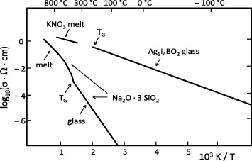
Figure 25. Ionic conductivities of vitreous ionic conductors. Redrawn after Ingram [106].
Download figure:
Standard image High-resolution imageFigure 25 is meant to convey an idea of the wide range of glass-forming systems which exhibit significant ionic conductivities, encompassing fast-silver-ion-conducting glasses such as Ag5I4BO2 [108] as well as conventional network glasses such as Na2O · 3SiO2. Obviously, the iodoborate glass has potential for use in room-temperature solid state batteries and other devices [165], while the silicate glass is more suited to high-temperature applications [166].
Note also the characteristic change in shape of the temperature-dependent conductivity that is seen for Na2O · 3SiO2 at its glass transition, where the coupled ergodic system (melt) transforms into the decoupled non-ergodic system (glass). In a later subsection, the difference between non-Arrhenius and Arrhenius conductivities will be considered in more detail.
Around 1980 conductivities such as those in figure 25 raised the question why activation energies varied so markedly. At that time European scientists, mostly in France, reconsidered the well-known model of Anderson and Stuart (USA) [167] and used it as a guideline for understanding the hopping mechanism in glass, with the aim of optimizing it. Simple chemical clues were provided by the Anderson–Stuart model, including the favorable effects of a polarizable and flexible matrix, i.e. of ion–matrix interactions. These basic criteria led to the synthesis of new glasses in which oxide ions were replaced by sulfide ions. Examples were the thio analogues of phosphates, silicates, etc as described by Ribes et al (France) [168] and by Malugani et al (France) [169].
Starting from glasses made of a network former (such as SiO2 or B2O3) and a network modifier (such as Na2O or Ag2O), ionic conductivities could be further increased by doping with a salt (such as NaCl or AgI). An example is the silver iodoborate glass of figure 25, since 8AgI · Ag2O · B2O3 is just the same as two times Ag5I4BO2.
This dopant salt concept was a French invention, coming out of Bordeaux [157] and Grenoble and Montpellier [158]. Almost two decades later, the effect was revisited by Swenson and Börjesson (Sweden) [170], who related the relative increase in conductivity, Δ σrel = (σdoped - σ0 )/σ0, to that in network volume, ΔVrel = (Vdoped - V0 )/V0, and thus discovered a cubic power law, Δ σrel ∝ Δ Vrel3. In a log–log plot of σdoped /σ0 ≈ Δ σrel versus Δ Vrel, as reproduced in figure 26, this corresponds to a straight line with a slope of three.
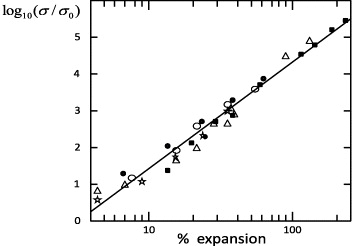
Figure 26. Relative conductivity, σ /σ0, where σ0 is the ionic conductivity of the undoped glass, versus the expansion of the glass-network forming units, (Vdoped - V0 )/V0, for various salt-doped glassy electrolytes. Redrawn after [170].
Download figure:
Standard image High-resolution imageSeveral groups in France [171], Italy [172] and the UK [173] studied the effects of pressure on doped and undoped Ag+-conducting glasses and thus determined the respective activation volumes (VA) for silver-ion transport. A striking result emerged. In the undoped glass (AgPO3) the activation volume turned out to be essentially the cationic volume of about 5 cm3 mol−1. On the other hand, doping with either AgI or Ag2S led to a marked reduction in VA, i.e. to a value of about 2.3 cm3 mol−1. This effect was found to be linked to a commensurate reduction in activation energy.
Another phenomenon, which was put on the map in the mid-1980s by Minami's group at Osaka (Japan) [174] and also by Deshpande et al (France) [175], was the so-called mixed glass-former effect. Replacement of one glass former by a combination of two was found to give rise to increased conductivities, see also later papers of the Montpellier group [176, 177].
At this point let us once again go back in history. Even before E Warburg discovered ionic transport in glass, attention had already been drawn, also in Germany, to a puzzling effect that became known as the thermometer anomaly and eventually turned out to be caused by ionic motion in glass as well. When a calibrated thermometer made of Thuringian glass was put into boiling water and later into ice of 0 °C, it would show - 0.5 ° C instead of 0 °C, the 'zero-point depression' vanishing only after several months. In 1883, R Weber found out that the effect could be reduced by a factor of ten if, instead of sodium and potassium, only one kind of alkali ion was present in the glass [178]. Evidently, the presence of both alkalis impeded the structural rearrangement that was required for the contraction of the glass upon cooling. A little bit later Otto Schott, Jena (Germany), developed the first accurate lithium-based thermometer.
Since Schott's times, it has become apparent that the thermometer effect belongs to a larger class of phenomena, now known as the mixed alkali effect (MAE). The most prominent of these anomalies is the unexpectedly pronounced minimum of the ionic dc conductivity in mixed-alkali glasses, which was first reported by Gehlhoff and Thomas (Germany) in 1925 [179]. For reviews, see Isard (UK) [180], Tomandl and Schaeffer (Germany) [181] and Ingram (UK) [159].
Obviously, the MAE in glass and the mixed-cation effect in β-alumina are related phenomena. Indeed, they have been traced back to similar origins, with site preferences playing the essential role. There is, however, a subtle difference. In the crystalline case, the different ionic species prefer crystallographically non-equivalent sites on an existing lattice, while in the vitreous case they create their own characteristic environments when the glass is formed from the melt.
The existence of ion-specific sites in glass was clearly shown in the classic extended x-ray absorption fine structure (EXAFS) work of Greaves et al (UK) [182] who obtained distinct radial distribution functions for different kinds of ions, irrespective of the actual glass composition. As exemplified in figure 27, potassium ions and cesium ions tend to retain their characteristic environments, as observed in their respective single-alkali silicate glasses, even in a mixed glass of composition KCsSi2O5.

Figure 27. Fourier transforms of weighted EXAFS spectra from three alkali silicate glasses, redrawn after [182].
Download figure:
Standard image High-resolution imageThe crucial results of Greaves et al led Maass, Bunde and Ingram (Germany and UK) to develop their dynamic structure model (DSM) [183, 184], in which they described the hopping motion of ionic species in glass via pathways formed by their own appropriate sites.
The main features of the MAE could, indeed, be replicated on the basis of the DSM, by considering suitable pathways for alkali ions A+ and B+ in glasses of composition y(xA2O(1 − x)B2O)(1 − y){SiO2, B2O3, ...}, which form spontaneously in the glass in response to the movement of the cations [184].
The predictions based on the DSM included the following. If a fraction of the sodium ions in a sodium-ion-conducting glass were replaced by silver ions, a structural change could be effected by the mobile Ag+-ions even at a temperature, say, 200 K below the glass transition. In fact, this has been confirmed by studies both in Germany by EXAFS [185] and in the UK and Greece by infrared reflection spectroscopy [186]. On the other hand, recent studies, again in Germany [187] and the UK [188], have shown that a 'normal' MAE is not established when K+-ions are introduced into a sodium silicate glass, even slightly above TG. Clearly, the opening up of potassium sites is inhibited by the compressive stress caused by the size of the K+-ion. Rather, compressed layers are thus formed, providing the basis for an industrial process for the chemical strengthening of glass.
In the case of single-alkali glasses of composition yA2O(1 − y){SiO2, B2O3, ...}, the authors [184] were able to use their model to reproduce the empirical power-law dependence of the dc conductivity on y, σ ∝ yconst, which is equivalent to a logarithmic dependence of the dc activation energy on y,  . In yNa2O(1 − y)B2O3 at 150 °C, for instance, the dc conductivity increases by more than seven orders of magnitude, when y is increased from 0.1 to about 0.4 [189, 190].
Souquet et al [191] (France) have shown that the activation volume for Na+ transport in a sodium-ion-conducting glass is close to the ionic volume of about 5 cm3 mol−1. In a British–German collaboration, an increase of VA has however been observed upon gradual reduction of the sodium fraction in a borate glass [192]. Obviously, it becomes harder to open up new sodium sites, if the glass is alkali-poor. The effect is even more clearly visible in mixed-alkali borate systems [193].
The pressure dependence of the hopping dynamics of the Rb+-ions in a rubidium borate glass was studied experimentally at Aberdeen (UK) and Münster (Germany). Pressure was thus shown to affect the coefficient of self-diffusion of the Rb+-ions more strongly than the ionic conductivity [194]. Indeed, the Haven ratio5 was found to become as low as 0.02 at 6 kbar. On the basis of linear response theory, the effect was explained by pressure favoring a positive directional correlation of the hops of neighboring ions, in the sense of a caterpillar mechanism [194, 195].
While EXAFS has been successfully applied for studying the immediate neighborhood of mobile ions in glass, x-ray and neutron diffraction data have shown that the framework atoms of glasses also possess well-defined nearest-neighbor environments, thus constituting short-range order [196–199]. In AgI-containing glasses, medium-range effects have been revealed by the group at Besançon (France) [200] suggesting that 'clusters' or 'connecting tissues' of AgI might provide the preferred pathways for Ag+- migration, on tracks formed by the iodide ions.
At the same time, advanced NMR techniques have been used to elucidate relevant structural details on a somewhat larger scale, i.e. those features that are characteristic of medium-range to long-range order. In a recent review by Brunklaus et al [201] (Germany) mention is made of many applications of solid state NMR in the field of vitreous electrolytes.
For instance, the technique of magic-angle spinning NMR has been applied to a huge variety of oxide glasses, providing a possibility to identify structural units that contain different numbers of non-bridging oxygen ions and to quantify their respective fractions [202]. Techniques such as SEDOR (spin echo double resonance) and REDOR (rotational echo double resonance) have been employed to investigate spatial cation distributions [203], correlations between network formers and network modifiers [204], as well as network former connectivities [205]. The latter topic is relevant for explaining the mixed glass-former effect.
The following interesting insights have been obtained by molecular dynamics (MD) simulations performed in the group of Heuer (Germany). Clearly, there would be a marked increase in the activation energy for ionic transport, if the glassy network was not allowed to relax [206]. This result emphasizes once again the importance of ion–matrix interactions. Structural disorder in glass was often thought to imply that, in analogy to crystalline fast ion conductors such as α-AgI and α-RbAg4I5, the number of available vacant sites exceeded the number of ions of the mobile kind. However, results obtained by Heuer's group from MD simulations rather suggest that there are (many) more occupied sites than vacant ones [207].
8.3. Universal features of frequency-dependent ionic conductivities
In the last few decades, ion-conducting glasses (as well as many other solid electrolytes) have been found to show an unexpected degree of similarity in their broadband conductivity spectra. In particular, two surprising 'universalities' have been detected, see figures 28 and 29. One of them, the first universality, has turned out to be a fingerprint of activated hopping along interconnected sites, while the other, the second universality, also known as nearly constant loss (NCL) behavior, reflects non-activated, strictly localized movements of the ions. The former is observed at sufficiently high temperatures, while the other is found at sufficiently low ones, e.g. in the cryogenic temperature regime.
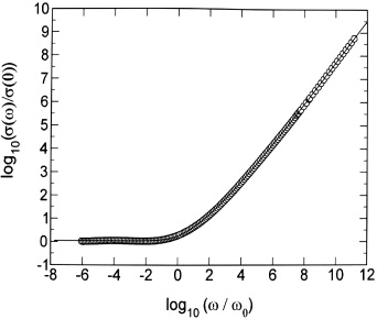
Figure 28. First universality. This scaled representation of experimental and model conductivities (circles and solid line, respectively, with data from 0.45 LiBr · 0.56 Li2O · B2O3 glass) is characteristic of many disordered ion conductors which largely differ in phase, structure and composition. Note that the slope increases continuously, slowly tending toward unity [195, 208]. The onset of the dispersion is slightly more gradual in mixed alkali glasses and in materials with low dc conductivities, see [209, 210], respectively.
Download figure:
Standard image High-resolution image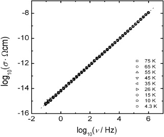
Figure 29. Second universality (nearly constant loss). Low-temperature conductivity isotherms displaying a linear frequency dependence and essentially no temperature dependence (data from 0.3 Na2O · 0.7 B2O3 glass) [195, 211].
Download figure:
Standard image High-resolution imageThe fascination of the two universalities lies in their ubiquity, i.e. in the occurrence of either or both of them in quite different kinds of disordered ion-conducting materials [195]. These include crystalline, glassy and polymer electrolytes, molten salts and ionic liquids. Evidently, the existence of the universalities is not primarily a consequence of phase, structure and composition, but rather of some common laws that govern the many-particle dynamics of the mobile ions.
The initial step toward our present notion of the first universality was taken in London, in 1975, when Jonscher [145, 146] discovered what he called the universal dielectric response or the universal dynamic response, abbreviated as UDR. Based on a huge collection of frequency-dependent conductivities of ion-conducting materials, he introduced his famous power-law description, σ (ν ) - σ (0) ∝ νp.
Later on, authors in many countries applied the power law to fit their experimental data, see for instance [134, 144] and the example of figure 23. They often made their spectra collapse into one, as in figure 28, by means of Summerfield scaling [147], which is the most frequent case of time–temperature superposition of conductivity spectra [212–214]. In the meantime, however, it has become apparent that Jonscher's power-law approach is at variance with both experiment and theory [215, 216].
Shortly after Jonscher's findings, Ngai (USA) formulated his coupling concept [217–219], which emphasized the importance of ion–ion interactions without violating linear response theory. However, the coupling concept still employed a power law in order to describe the increase of σ (ν ), before a high-frequency plateau, σhf, was eventually attained.
In their Monte Carlo studies, Bunde et al (Germany) considered the effects of structural disorder and long-range Coulomb interactions systematically [220–222]. In particular, they reproduced the frequent occurrence of correlated forward–backward hopping sequences, which is the main cause of the first-universality phenomenon. Disorder and interactions were also taken into account in the counterion model developed by Dieterich et al (Germany), who derived realistic spectra, σ (ν ), from their numerical simulations [223, 224].
The random barrier/random energy models have also been devised in Europe, namely by Dyre and Schrøder in Denmark [225–228] and by Baranovski and Cordes in Germany [229]. These authors modeled the non-random ion dynamics in a formal fashion by considering individual mobile ions in random potential landscapes that are static in time, again obtaining realistic shapes of σ (ν ).
The alternative viewpoint was to assume that the site potentials of the ions were not static, but varied in time, thus reflecting their changing momentary arrangements and interactions. This view led to the construction of a series of jump relaxation models by Funke et al (Germany). On the basis of Debye–Falkenhagen-type arguments, see one of the previous subsections, simple coupled rate equations were formulated to describe the ion dynamics [140, 208]. The solid line in figure 28 has been derived from the most recent model version, called the MIGRATION concept [195, 230], the acronym standing for MIsmatch Generated Relaxation for the Accommodation and Transport of IONs.
The essential message contained in broadband conductivity spectra, which may cover more than 17 decades on the frequency scale [231], is the following. Many 'elementary' hops of the mobile ions are seen (per unit time) within a sufficiently short time window, corresponding to the hf plateau of the conductivity. Eventually, however, only a small fraction of them prove 'successful', contributing to the dc conductivity and thus constituting the long-time 'random' hopping dynamics of the ions. In glassy and structurally disordered crystalline electrolytes, the 'elementary' hops as well as the fraction of 'successful' ones are usually Arrhenius activated.
In 1991, Nowick and his co-workers (USA) [232] discovered a new 'universal' feature, now called second universality. The phenomenon is ubiquitous in disordered ionic materials ('present in every plastic bag'), but becomes visible only at sufficiently low temperatures and/or high frequencies. The expression nearly constant loss (NCL) refers to the dielectric loss function being virtually independent of both frequency and temperature, ε '' ∝ σ /ν = const, cf figure 29.
There has always been a broad consensus that the second universality reflects cooperative localized movements of a large number of ions. Remarkably, the advancement of a more detailed modeling has been quite similar to the progress made in understanding the first universality. Again, early interpretations were based on the assumption of specific static distributions of the potentials felt by the mobile ions [233, 234], while more recent investigations have shown that this assumption was unnecessary. Indeed, the effect could be traced back to a time dependence of the single-particle potentials, produced by Coulomb interactions [195, 208, 211, 235–237].
The decisive step forward was taken in 1998, when Dieterich and his co-workers (Germany) treated the locally mobile ions as reorienting electric dipoles, with Coulomb interactions between them. In their Monte Carlo studies, they considered random collections of such dipoles and studied their localized reorientational movements [235, 236]. As a result, they obtained a linear NCL regime in σ (ν ), lying between two crossover points. The frequency range spanned by the NCL was found to increase as the ratio of Coulomb energy by thermal energy was increased, i.e. with increasing number density and with decreasing temperature.
Similar results have also been derived from a suitably modified version of the MIGRATION concept [195, 208]. According to this treatment, the Coulomb interactions seem to create rapid see-saw-type variations of the local potentials experienced by the individual ions, resulting in non-activated collective localized movements [237].
8.4. Polymer electrolytes
In the evolving scheme of figure 21, glassy electrolytes are followed by ion-conducting polymers. These constitute a broad class of materials that are in many ways even more demanding than the glassy systems, for instance, with regard to their structures and their ion dynamics. A specific new complication arises above the glass transition temperature, TG, where the concept of a stable matrix must be abandoned and where the absence of fixed sites makes a visualization of the motion of the mobile ions almost impossible. On the other hand, the potential of ion-conducting polymers for applications in all-solid-state devices, see below, has greatly spurred their further development since the time of their discovery in the mid-1970s.
In 1975, Peter V Wright [238], a polymer chemist from Sheffield (UK), produced the first polymer electrolyte by employing polyethylene oxide (PEO) as a host for sodium and potassium salts. Michel Armand (France) immediately realized the big advantage that salt-in-polymer electrolytes such as, for instance, lithium-PEO would offer in electrochemical cells, ensuring permanent contact between electrode and electrolyte materials upon cycling [239, 240]. The mechanically soft and flexible polymer would, indeed, provide excellent interfacial contact even with intercalation-type electrodes whose volumes vary considerably during charging and discharging.
The ionic conductivities reported by Armand et al [240] were only about 10−5 Ω−1 cm−1 at 40 °C to 60 °C, which was clearly less than what could be achieved in a glass. However, it was also realized that this could largely be compensated for by a thin-film cell configuration.
More specifically, PEO complexes containing thiocyanides of sodium and potassium, NaSCN and KSCN, were shown to exhibit different temperature dependences of their ionic conductivities above and below about 330 K [240]. Below that temperature, the dc conductivities were well reproduced by the Arrhenius law, hinting at charged defects moving via a hopping mechanism. At higher temperatures, the NaSCN-containing complex was found to follow the Arrhenius law again, but with a smaller activation energy, while the conductivity of the complex with KSCN could be well described by the empirical VTF equation [112–114], σ (T)∝exp (-(Ea/kB)/(T-T0)). It was concluded that the NaSCN-containing complex was crystalline on either side of the transition, as shown in figure 30, with particularly easy formation of mobile cation vacancies in the high-temperature modification. On the other hand, the validity of the VTF equation for the KSCN containing complex was interpreted in terms of a free-volume-type model [241].

Figure 30. Structure of crystalline PEO complexes, according to [240], by courtesy of Michel Armand. (a) Low-temperature stoichiometric form and (b) high-temperature defective form.
Download figure:
Standard image High-resolution imageFour years later, however, on the basis of their more recent NMR results, Berthier, Armand and co-workers [110] (France) arrived at a quite different conclusion. Having analyzed different salt-in-polymer electrolytes and having always noted a considerable reduction of the fraction of crystalline material at the transition from highly activated to easy ion transport, they inferred that it is only the non-crystalline elastomeric material that is responsible for the motion of the mobile ions. The idea put forward in [110], i.e. that only an amorphous polymer host would support fast ion transport, was soon considered a paradigm of polymer research.
In the decades to follow, pronounced segmental motion and flexibility were, therefore, considered the prime guidelines in search of polymer electrolytes with high ionic conductivities. The results obtained have been documented in a number of reviews, many of them by European authors [242–248].
Here we note that the measurement of ionic transference numbers in polymer electrolytes, see Bruce et al (UK) [249], as well as the enhancement of the observed steady-state currents by diffusing ion pairs, see Cameron et al (UK) [250], were important topics in the late 1980s.
Besides salt-in-polymer complexes with different host polymers and different salts dissolved in them, polyelectrolytes were identified as another promising group of ion conductors with polymer structures. In these, the polymer itself is (for instance, negatively) charged, while the counterions (for instance, Li+ ions) are free to move [251]. In comparison with salt-in-polymer complexes, polyelectrolytes thus have the advantage of not suffering from the unfavorable effect that the formation of ion pairs can have on the ionic conductivity. For a systematic investigation of ion pairing, both experimental and theoretical, see a recent mini-review by Stolwijk et al (Germany) [252].
Regarding salt-in-polymer systems that fulfill the requirements of high ionic conductivity and mechanical strength as well as chemical, thermal and electrochemical stability, progress has been made along different routes.
In the first place, new polymer architectures have been introduced, such as star-branched PEO–salt complexes, see for instance a recent paper by the Warsaw group [253], as well as modified PEO main chains with grafted polymers. For instance, comb-branched block copolymers [254] and cross-linked polymer networks [248] have been found to offer favorable mechanical and electrical properties. This includes polymer electrolytes based on polyphosphazenes [255–258] and polysiloxanes [258–261], as investigated especially by the groups of Wiemhöfer (Germany) and West (USA).
Another successful approach, which had been demonstrated for crystalline electrolytes earlier (see the following subsection), was suggested by Weston and Steele (UK) in 1982 [262] and by Wieczorek et al (Poland) in 1991 [263]. These authors prepared salt-in-polymer systems with finely dispersed micro- or even nano-sized ceramic filler particles. Significantly enhanced ionic conductivities were thus attained, the effect clearly increasing with decreasing particle size, as shown in 1998 by the group of Scrosati (Italy) [264].
The characteristic VTF-type temperature dependence of ionic conductivities that is displayed by polymer electrolytes at temperatures well above the glass transition temperature [240, 265], and also by fragile molten salts and ionic liquids [111], has often been explained in terms of either free volume [241, 266, 267] or configurational entropy models [268, 269].
More recently, however, a novel route has emerged for deriving the long-time behavior of the mobile ions from their short-time dynamics, and thus to model temperature-dependent dc conductivities. A typical result is shown in figure 31.
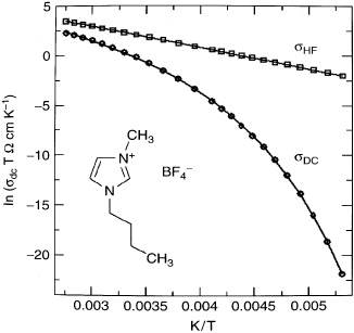
Figure 31. Dc and hf conductivities of the ionic liquid 1-butyl-3-methyl-imidazolium tetrafluoro-borate. The experimental dc data are complemented by Arrhenius-activated model values at high frequencies, where every elementary displacement is registered. The solid lines result from the modeling of [195, 270]. The figure is taken from [271], with permission from Wiley-VCH.
Download figure:
Standard image High-resolution imageThe basic argument, developed by the Solid State Ionics group at Münster (Germany) [195, 270], is the following. The conductivities of glasses, ionic liquids and polymer electrolytes rather unexpectedly display the same first-universality features on the frequency scale. As regards the temperature dependence, however, there is an important difference between glasses and 'non-Arrhenius' materials. After a thermally activated elementary displacement of a mobile ion, its immediate backward motion appears to be non-activated in the 'non-Arrhenius' materials (while it is activated in a glass). Therefore, the position of the high-frequency end of the dispersion of the conductivity, marking the inverse of the time when backward ('roll-back') movement sets in, does not depend on temperature. As a formal consequence, ln(σhf /σdc) is found to increase with inverse temperature in an exponential fashion, see figure 31.
The resulting dc conductivity is indeed very close to VTF. Good fits have been made also for the conductivities of various polymer electrolytes [272].
In the new millennium, the paradigm introduced in 1983 by Berthier and Armand [110] was surprisingly overturned, when the group of Peter Bruce at St Andrews (Scotland, UK) proved that high ionic conduction was very well possible in crystalline polymer hosts [273–276]. The first crystalline polymer–salt complexes that were shown to support ionic conductivity were PEO6:LiXF6, where X could be P, As or Sb [273]. A significant further increase of the ionic conductivity was then achieved by the partial replacement of the anions, for example by N(SO2CF3)2− ions, see figure 32 [274], or by doping the polymer itself [275], or by using small-molecule electrolytes, Gn:LiAsF6, with Gn standing for CH3–O–(CH2–CH2–O)n–CH3, with n = 3 or 4 [276].
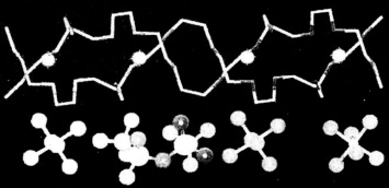
Figure 32. Fragment of the crystal structure of PEO6: (LiAsF6)1−x(LiTFSI)x according to [274]. In the figure, the AsF6− ions are partially substituted by bis(trifluoromethanesulphonyl)imide (TFSI) ions, N(SO2CF3)2−. The mobile lithium ions are contained in the polymer coil. Note the similarity to the concept of figure 30.
Download figure:
Standard image High-resolution imageMore recently, the group of Schönhoff and Cramer (Germany) analyzed the ionic transport properties of solid (yet non-crystalline) polyelectrolyte complexes such as the one sketched in figure 33. In these materials, the charge carriers are alkali ions in their hydrated state. Apart from the usual time–temperature superposition principle [212–214], the authors also detected a corresponding time–humidity superposition principle [277, 278], with the dc conductivity and the onset frequency of the dispersion depending exponentially on relative humidity.

Figure 33. Sketch of a solid polyelectrolyte complex of anionic poly(styrenesulfonate) containing Na+ and Cs+ as counterions and cationic poly(diallyldimethylammonium chloride); the Cs+ ion (on the left, with the smaller hydration shell) is more mobile than the Na+ ion (on the right); after [277, 278].
Download figure:
Standard image High-resolution imageIn 2009, the discovery of a rather unexpected crystalline fast-ion conductor with a polymer structure was reported by a group of Italian and Hungarian authors led by Riccò, Parma [279]. The ionic dc conductivity of the low-temperature phase (T < 400 K) of two-dimensionally polymeric Li4C60 [280, 281] was found to be as high as 0.01 Ω−1 cm at 30 °C, with an activation energy of only 240 meV. Passageways for the lithium ions between the fullerene balls are indicated in figure 34.
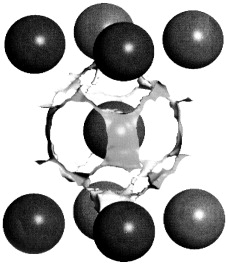
Figure 34. Illustration of possible paths for Li+ ion diffusion in polymeric Li4C60. Dark balls are fullerene molecules; according to [279].
Download figure:
Standard image High-resolution imageA stunning property of this polymeric electrolyte is the reported absence of any conductivity dispersion. Also, which is equivalent, its 7Li spin–lattice relaxation rate, when plotted versus inverse temperature, was found to be symmetric, in agreement with BBP theory [149]. A probable explanation is the following. There is hardly any Coulomb interaction between the mobile Li+ ions, if their electric charges are mostly shielded by mobile electrons in the fullerene molecules. The lithium ions would thus diffuse almost randomly within the regions of space available for them.
For a comprehensive review of the topic 'Polymer electrolytes, present, past and future', the reader is referred to a recent publication by Di Noto et al (Italy) [282].
8.5. Nanoionics
In nanosized systems such as nano-composites and thin films (level 3d), surfaces and interfaces play a paramount role in creating unexpectedly pronounced, sometimes even dramatic, ionic (and electronic) conductivity effects. For recent reviews on this topic, now known as nanoionics, see [117, 118, 283–289].
A particular example already mentioned in the preceding subsection concerned polymer electrolytes that were heterogeneously doped with nanosized ceramic materials such as SiO2 [262–264]. An even more spectacular effect had been discovered as early as 1973, when Liang (USA) [115] observed an increase of the ionic conductivity of the ionic conductor LiI by a factor of about 50, upon adding the insulating compound Al2O3 as a dispersed second phase. Similarly, Maier and co-workers (Germany) [116, 290] as well as Shahi and Wagner (USA) [291] reported on highly conductive pathways in Ag- and Tl-halides that were created by the introduction of nanosized Al2O3 particles.
Early on, the counter-intuitive phenomenon of a conductivity enhancement that was achieved by adding an insulating second phase could be explained in terms of a space-charge model [116], which adopted and extended ideas that had been developed previously by Carl Wagner for the purely electronic case [292]. A thorough discussion of this model, amounting to a detailed description of how the defect chemistry is modified in space-charge regions in front of interfaces, was given by Maier in 1995 [293]. In 2003, the same author introduced the energy level representation of figure 35 for an elegant visualization [118].
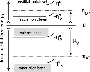
Figure 35. Energy level diagram for a mixed conductor MX with Frenkel disorder in the cation lattice, showing level bending at the equilibrium contact to a second phase. Top: ionic disorder. Bottom: electronic disorder in upside-down representation. The chemical potential of M is indicated by the two-headed arrow on the right-hand side. Redrawn from [118, 294].
Download figure:
Standard image High-resolution imageAlthough the ionic levels included in figure 35 may look less familiar than the electronic ones, they clearly display analogous behavior. Basic relationships can be read from the diagram. The most important aspect is, of course, the constancy of the electrochemical potentials of metal ions and electrons in the region of varying electric potential. Note also that the electric energy terms cancel in the sum of the electrochemical potentials, so that ηM+ + ηe- and the chemical potential of M, which is μM = μM+ + μe-, become identical. They also cancel in the distance of the two ionic levels from each other. In explicit building-element notation this distance is the sum,  , while in 'shorthand notation', cf figure 35, with indices i and V standing for 'interstitial' and 'vacancy', respectively, it is
  . This finally becomes
  , because of the equilibrium condition, which is Δ GFrenkel = μi + μV = 0.
In the absence of any non-zero electric potential, the level of ηM + is found to be situated at a distance of  below ηi ° and at a distance of
  above - ηV °. However, if positive charges are accumulated at the interface, this will result in a position-dependent electric potential and thus in a level bending as shown in the figure. Consequently, cation vacancies will be enriched and interstitial ions will be depleted in the space-charge zone in front of the interface.
In the case of heterogeneous doping of LiI with Al2O3, Li+ ions are adsorbed on the oxide's surface. As a result, lithium vacancies are enriched in front of the interface, providing highly conductive pathways, as pointed out by Maier in 1995 [293]. In the group of P Heitjans (Germany), the same effect has been seen in a nano-composite system consisting of Li2O and B2O3 [287]. An NMR line measured on such a sample at a given temperature is reproduced in figure 36. Evidently, it consists of two components. One of them is motionally narrowed, while the other is not, the former being caused by highly mobile lithium ions located in the interfacial regions, the latter being due to less mobile lithium ions within the crystallites.
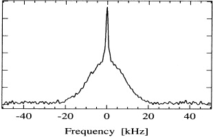
Figure 36. 7Li NMR lineshape at 58 MHz and 433 K of nano-crystalline 0.5 Li2O · 0.5 B2O3, taken from [287]. By courtesy of Heitjans and Indris.
Download figure:
Standard image High-resolution imageMany more examples can be given. These include the effects of grain boundaries in both cation and anion conductors. For instance, grain boundaries in AgCl adsorb silver ions and thus create mobile silver vacancies in front of them [294]. Likewise, fluoride ions are accumulated at grain boundaries in CaF2, which leads to increased anionic conductivity due to fluoride vacancies in the space-charge region [295, 296].
In nano-crystalline materials, the interfacial effects may completely dominate. A particularly nice example, studied in the laboratories of Tuller (USA) [297], Birringer (Germany) [298] and Maier (Germany) [299], is ceria, CeO2, which is homogeneously (but only weakly) doped with some heterovalent acceptor, i.e. with some oxide A2O3. If the material is coarse-grained, it contains a large number of oxygen vacancies, but only few excess electrons, and exhibits oxygen conduction. However, when prepared in nano-crystalline form, the material becomes an electronic conductor. This is a consequence of positive charges assembling at the grain boundaries, causing a substantial enhancement of electron density and a concurrent decrease in oxygen vacancy density in the immediate neighborhood [297–299]. Figure 37 is meant to visualize the transition from the bulk to the near-interface properties [299]. In the figure, the size of the grains is still larger than the Debye length, λ, which is a rough measure of the extent of the space-charge layer.

Figure 37. A nanosized block of acceptor-doped ceria, (1 − x) CeO2 · x A2O3, after [299]. In the bulk, the oxygen vacancies by far exceed the free electrons in number density, but this is reversed in the immediate vicinity of the grain boundary.
Download figure:
Standard image High-resolution imageGenerally, the number densities of the defects, as indicated in figure 37, are obtained by first solving the Poisson–Boltzmann equation (perpendicular to the grain boundary) for the electric potential and then transforming the potential variation in this direction into the variations of the number densities of the defect species. In the case of the figure, which is termed Gouy–Chapman [300, 301], the decisive defects are supposed to be mobile and to be suitably redistributed upon introduction of an electric-potential gradient. It is, however, also conceivable that the dopant ions are not mobile, their number density remaining spatially constant. This is the Mott–Schottky case, which results in different shapes of the densities of the other defects [302–304].
In a recent analysis of lateral conductivities of nano-sized multilayer heterostructures of CaF2/BaF2, both kinds of space-charge profiles were identified in Maier's group at Stuttgart (Germany) [305]. The significant conductivity increase that had been measured as a function of inverse interfacial spacing could, indeed, be explained by Mott–Schottky/Gouy–Chapman situations at low/high temperatures, respectively.
In thin-film systems, lateral conductivities increase with inverse film thickness because the space-charge layers occupy an ever larger fraction of the cross section. This size effect has been called 'trivial', as long as the film thickness is well above 4λ, with the space-charge regions not extending to the center of the film. Another, 'true' size effect is, however, observed at thicknesses well below 4λ, when the space-charge regions overlap and the intrinsic bulk behavior has completely disappeared [54, 118, 288].
9. Solid State Ionics, from 1972 onward: an international endeavor
Back in 1960, Takehiko Takahashi (Japan) had introduced the very term 'Solid State Ionics' to represent the emerging field of solid electrolytes [306]. In international common usage, however, expressions such as 'solid electrolytes' and 'fast ion transport in solids' continued to be more customary. They were replaced by 'Solid State Ionics' only about two decades later, when the proceedings of the Tokyo Solid State Ionics conference (1980) were published in the journal Solid State Ionics.
The first international conference on this topic was held at Belgirate, Italy, in September 1972. The symposium was organized in the form of a NATO Advanced Study Institute on 'Fast Ion Transport in Solids, Solid State Batteries and Devices'. Undoubtedly, the most renowned scientist attending was Carl Wagner. The Belgirate conference proceedings, edited by the organizer, van Gool (The Netherlands) [307], were published in the following year.
Notably, the solid electrolytes used up to the time of the Belgirate meeting had mostly been based on, or related to, AgI and doped ZrO2; the beta alumina family had been discovered only a few years prior to the meeting. In van Gool's own words, the most important achievement of the conference was that scientists, until then working as individuals, formed a nucleus that was going to shape the field of solid electrolytes in the years to come6.
In retrospect, the Belgirate conference is indeed remembered for marking a point in time when Solid State Ionics became a truly international endeavor, with scientists in many countries closely cooperating and, as it were, setting out to new shores. The new initiatives taken included in particular the quest for new materials and new technologies.
Regarding new materials, the impression conveyed at Belgirate was that 'we have only scratched the surface'7. The truth of this assessment was to become obvious in the decades to follow. Regarding new technologies for possible applications, the message was twofold. On one hand, a long list of devices could be envisaged, including not only batteries, fuel cells and sensors but also ionic pumps, ion-transport membranes and ionic capacitors with high power densities. On the other hand, it was only realistic to foresee that considerable technological problems would be awaiting along the way.
A series of four international meetings on 'Fast Ion Transport in Solids' was initiated by the Belgirate Advanced Study Institute. The second and third were conferences held in the United States, namely at Lake Geneva, Wisconsin, in 1979 and at Gatlinburg, Tennessee, in 1981. The fourth meeting in the series was again held at Belgirate, Italy, marking the 20-year anniversary of the first, in 1992. Scrosati (Italy) was instrumental in organizing it as an Advanced Research Workshop, again sponsored by NATO, at the same location on Lago Maggiore and again in the month of September.
Comparison of the proceedings of the second (II) Belgirate meeting [308] with those of the first (I) highlights the major lines of development taken by Solid State Ionics during those 20 years as well as the large body of work completed. To cite Bruce (UK)8, 'Topics that were central or even dominant in the field in 1992, such as intercalation electrodes and polymer electrolytes, had been in their infancy or not yet born in 1972'.
While polymer electrolytes had in fact been unknown in 1972, the intercalation concept had just come into existence. At the Belgirate I conference, it was presented independently by Steele (NaxTiS2) from the UK9 and by Armand (graphite-CrO3) from France10. One year earlier, compounds showing intercalation-type behavior, namely tungsten and vanadium bronzes, had been described by Whittingham and Huggins (USA) [309], and a few years later Whittingham [310] was the first to demonstrate the use of the intercalation compound LixTiS2 as a cathode in a rechargeable lithium battery. At the Belgirate II meeting, Bruce reported on the diffusivity of Li+-ions in both layered and cubic TiS2 and proposed a mechanism for electrointercalation (see footnote 8). At the same meeting, the Bordeaux (France) group of Hagenmuller and Delmas introduced a lithium battery for electrical engine vehicles, in which reversible 'rocking chair' intercalation processes were occurring at both electrodes11.
Glassy electrolytes, pioneered at Belgirate I by Kunze (Germany) [163], had by 1992 developed into a well-established class of materials, and a large number of experimental studies on them was reviewed by Magistris (Italy)12.
The interesting possibility of a paddle-wheel-type interaction between translationally mobile cations and rotationally mobile anions, e.g. in the plastic-crystalline high-temperature phase of Li2SO4, was discussed at Belgirate II by Lundén (Sweden)13. This idea had first been suggested in 1989, by Lundén and Thomas (Sweden) [311]. On the basis of time-resolved experimental results for the localized cationic and anionic movements, the paddle-wheel mechanism could later be redefined for α-Na3PO4, see e.g. Wilmer et al (Germany and France) [312] and Witschas et al (Germany) [313].
Interfacial phenomena, in particular the kinetics of ion-transfer across interfaces, had already been discussed at Belgirate I, e.g. by Pizzini (Italy)14. However, the key role of ion-exchange kinetics at interfaces, in particular at the electrodes of solid state electrochemical cells, was perceived only at Belgirate II, see for instance the contribution by Boukamp et al (The Netherlands) on the surface oxygen exchange kinetics of solid oxide ion conductors15.
As pointed out by Weppner (Germany)16 at Belgirate II, the role played by electronic charge carriers in solid ionic and mixed conductors had previously been underestimated. An excellent and comprehensive treatment of the topic 'ions and electrons in solids' was given later by Maier (Germany) [54], cf also his energy-level diagram of figure 35.
Many more steps of progress in the development of Solid State Ionics have been reported at other meetings, some held before, but most of them after Belgirate II. These include in particular the biennial Solid State Ionics series of international conferences.
At one of those Solid State Ionics conferences, held at Monterey, California, in 2003, Joop Schoonman (The Netherlands) gave a most memorable opening address, drawing the attention of the audience to the increasing awareness of environmental factors and limited energy resources, which had led to a profound evolution in the way energy was generated, converted and stored. Schoonman's central sentence was this [314]: 'If there is one field that contributes to the search for materials for clean energy, it is our field of Solid State Ionics'. This sentence has since been considered a guideline for many activities in the Solid State Ionics community. The clean-energy environmental issue has indeed spurred the development of new functional materials and solid state electrochemical devices.
10. Functional materials and solid state electrochemical devices
10.1. Setbacks and success stories
In the field of applied Solid State Ionics, the years and decades after 1970 saw both setbacks and instant success stories. On one hand, the hopeful expectations regarding new battery systems, which had been raised by the discoveries of rubidium silver iodide and the beta aluminas, gradually gave way to more realistic views and solutions. On the other hand, solid electrolytes got successfully employed in cardiac pacemaker batteries and in lambda probes for automobile exhaust sensors. Both devices are now used around the globe and have thus drawn worldwide attention to applied Solid State Ionics. Although some of these lines of development had their origins outside Europe, all of them are certainly remarkable from a European perspective as well and will, therefore, be briefly sketched in the following.
Cells and batteries based on the fast silver-ion conductor rubidium silver iodide, RbAg4I5, such as Ag|RbAg4I5|RbI3, C, where Rb2AgI3 is formed in the cell reaction, were tested by Owens [315] (USA) around 1970. These cells were capable of operation at both high and low current density and over a wide range of temperatures. However, they suffered from rather low energy content per unit weight (about 5 W h kg−1) and have, therefore, never been commercially developed [316].
In contrast to RbAg4I5, lithium iodide, LiI, is a poor ion conductor, with a conductivity of only about 10−7 Ω−1 cm−1 at room temperature [317]. Nevertheless, this did not prevent the successful development of all-solid-state cardiac pacemaker batteries employing this solid electrolyte. To cite Owens [318], 'It was in Italy, in March 1972, in the city of Ferrara that for the first time a cardiac pacemaker, powered by a Li|LiI|I2 battery, was implanted into a human being'. Since then, the LiI battery has established an excellent record in reliability. Indeed, millions of persons have benefitted from implantable pacemaker devices containing LiI batteries [318].
The undoped lithium iodide was later replaced by LiI containing dispersed particles of Al2O3 as a second phase, resulting in considerably enhanced ionic conductivities [115]. Early on, iodine-PVP, PVP standing for poly(2-vinyl-pyridine), was identified and used as well-adapted electronically conducting cathode material [319]. Between this cathode and the lithium-metal anode the thin LiI film was formed by an in situ reaction. This offered the advantage of 'self-healing', with new lithium iodide being formed once cracks occurred in the solid electrolyte.
Sodium-sulfur cells, with ceramic beta alumina serving as solid electrolyte between the molten-sodium anode and the molten-sulfur cathode, were for a long while regarded as promising units for electrotraction, since they offered energy densities and, therefore, automobile operating ranges that surpassed the possibilities of conventional lead–acid or nickel–cadmium accumulators roughly by a factor of 10. The favored beta alumina variants included the lithium- and magnesium-stabilized sodium-β''-aluminas, which are similar to Na-β-alumina, but somewhat different in composition and structure [320, 321]. In Europe, the performance of state-of-the-art prototypes of the sodium-sulfur battery was presented and discussed at the 'International Workshop on Beta Aluminas and Beta Batteries', held at Druzhba, Bulgaria, in 1991 [322]. At that time real market introduction was still expected to be possible around the year 199517. Later, however, the further development of sodium-sulfur cells aiming at electrotraction was largely discontinued. The main reason was the unsolved problem of possible crack formation in the brittle solid electrolyte, entailing a catastrophic chemical reaction of molten sodium with molten sulfur. Here it is comforting that alternate forms of electrotraction, involving either lithium-ion batteries or fuel cells, are rapidly coming into view.
Remarkably, Solid State Ionics has provided a special gift for motorists, which Walther Nernst, who was an enthusiastic motorist himself, would have happily appreciated. Indeed, his two most prominent legacies, the Nernst equation and the Nernst mass, have been united in the concept of the lambda probe, which simultaneously serves the driver, the car and the environment.
The λ-probe, see figure 38, is an oxygen sensor based on the ceramic solid electrolyte YSZ (yttria stabilized zirconia). According to the Nernst equation, its e.m.f. (open cell voltage), E, is

Figure 38. Oxygen sensor based on the ceramic solid electrolyte YSZ as used in automobile λ-probes. The sketch is taken from [323] and refers to work done in H L Tuller's group at MIT (USA).
Download figure:
Standard image High-resolution imageHere, the oxygen activities on either side of the probe have been taken as a1 = p1 /p° and a2 = p2 /p°, with p1 and p2 denoting the oxygen partial pressures in the exhaust gas and in air, respectively. Obviously, the standard e.m.f. of the cell, E°, is zero, while the number of elementary charges involved per molecule of oxygen, |z|, is four.
As the oxygen partial pressure in air is sufficiently well defined, the oxygen partial pressure in the exhaust gas is given by the Nernst equation with sufficient accuracy as soon as the cell voltage has been measured. Figure 39 shows the variation in voltage as a function of the air–fuel ratio, λ. Note that the general shape reflects the principle of a titration curve. A near-zero signal corresponds to an oxygen-rich lean mixture and a voltage near 1 V to an oxygen-poor rich mixture. Because of the large step in voltage at λ = 1.0, which is the optimum value, the measured signal can be used to regulate the mode of operation of the engine's fuel injector in an unambiguous fashion.

Figure 39. Dependence of λ-probe voltage on air–fuel ratio. Note the strong deviation from the value at the stoichiometric point (λ = 1.0) that is observed if the mixture is too rich (λ < 1.0) or too lean (λ > 1.0). From [324], reproduced with permission of John Wiley & Sons, Inc.
Download figure:
Standard image High-resolution imageExhaust sensors of this kind, working in feedback mode with microprocessors and fuel injectors, have come to play an essential role in automobile construction, being installed in almost every automobile produced worldwide [323].
10.2. Sensors, smart windows and supercapacitors
It is worth mentioning that the lambda probe has found wide application as an oxygen sensor not only in car-exhaust systems but also in metallurgical and glass technologies, where the oxygen activity in the melt is an important process parameter, see for instance the book by Fischer and Janke (Germany) [325].
In 1980, M Kleitz and his group at Saint Martin d'Hères, France, reported on a cell which could be used as a potentiometric gas sensor both for oxygen in the absence of chlorine and for chlorine even in the presence of oxygen [326]. In this case, the reference electrode consisted of a layer of AgCl on silver, while the electrolyte was a composite chloride-ion conductor. The chlorine measurement could be performed down to 150 °C, while the oxygen measurement required somewhat higher temperatures. Three years later, again in France, a still different potentiometric oxygen sensor was proposed, which could be used at temperatures as low as 150 °C [327].
A potentiometric cell for monitoring the content of CO2 in air was developed by Holzinger, Fleig, Maier and Sitte (Germany) in the mid-1990s [328–330]. This remarkable sensor offered not only long-time stability and short response times, but could even be exposed to ambient atmospheres between 350 °C and 700 °C without sealing the electrodes. In the cell reaction, which is

CO2 is the only gaseous component, while the three solids are in their standard states. Therefore, according to the Nernst equation, the cell voltage is simply
In the cell, the above reaction is realized by sodium ions moving through the solid sodium-ion conductor Na-β''-alumina, while the solid components (plus Au) constitute the electrodes.
A quite different measurement principle has been employed in an oxygen sensor presented by the groups of Janek and Moos (Germany) in 2009 [331]. Like the lambda probe, the sensor is based on YSZ. Within the device, a temperature gradient is applied to a thick-film YSZ layer, and the resulting thermovoltage is measured. This measured voltage is found to depend on the oxygen partial pressure in a way that is in perfect agreement with theoretical predictions. The technique offers the advantages of little temperature dependence and no cross-sensitivity to a variety of other exhaust gases.
Electrolytic cells based on YSZ as a solid electrolyte may also be used to remove oxygen from stationary or streaming gas. Used for this application, first suggested by Yuan and Kröger [332], the device has become known as an oxygen pump. As reported by Yuan and Kröger, typical values of the attainable oxygen pressure are about 10−38 bar at 530 °C and 3 × 10⁻²⁷ bar at 800 °C.
While the electrochemical cells employed in cardiac pacemaker batteries and in lambda probes triggered the first truly international success stories in the field of Solid State Ionics, these have not remained the only ones. In the mid-1980s, a third such story was initiated in Europe, by the invention of the concept of 'smart windows' by Svensson and Granqvist (Sweden) [333, 334]. These authors proposed to exploit the electrochromic effect, described earlier by Deb (UK) [335], in devices that systematically modulate the light transmission of windows in the visible and infrared parts of the spectrum.
The aims pursued, the electrochemical background and the technical realization have all been set forth in a series of papers and reviews by Granqvist and his co-workers [336–340].
The predominant aim is to decrease the amount of solar radiation entering and heating up the inside of buildings (or cars) and thus to reduce the energy expenditure for air conditioning considerably. Another aim, relevant during the winter, is to let windows be transparent for visible light, but reflective in the infrared, thus blocking loss of interior heat.
In an electrochromic device, see figure 40, transparency to light is controlled by the darkening of a layer (electrochromic film) that occurs in a reversible redox reaction upon insertion of ions, for example lithium ions. This electrochromic material is typically tungsten oxide, WO3, and the reaction that causes darkening is

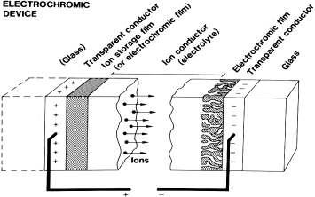
Figure 40. Basic design of an electrochromic device, indicating transport of positive ions under the action of an electric field, from [336], by courtesy of CG Granqvist.
Download figure:
Standard image High-resolution imageA solid lithium-ion conductor separates the electrochromic film from an ion-storage film, e.g. of LiCoO2, see figure 40. The two films consist of nanomaterials with well-developed nanoporosities, and the resemblance to a thin-film 'rocking chair' secondary battery is obvious. The outermost layers are transparent electrical conductors, typically of indium tin oxide, In2O3:SnO2 (ITO), and the overall transparency can then be controlled by an applied voltage [339]. Smart windows have meanwhile been tested and installed in different parts of the world, mostly for alleviating air conditioning loads by means of 'light balancing'.
Nanostructured, very large surface area electrodes are also essential in a novel class of electrochemical energy storage devices called electric double-layer capacitors or simply 'supercapacitors'.
The basic principle of supercapacitors consists in the formation of Helmholtz-type or, rather, Gouy–Chapman-type double layers in front of the very thin, nanostructured electrode material. The local situation is thus similar to the one presented earlier in figure 37. Note that the voltage drop in the capacitor is essentially across the double layers at the opposite electrodes which are rather close together, but separated by an ion-permeable membrane, the 'separator'.
The huge electrode surface areas, A, and the nano-sized thicknesses of the double layers, d, result in capacitances (proportional to A/d), which exceed those of conventional dielectric capacitors by orders of magnitude. Reported values are around or above 100 F g−1 for carbon materials such as aerogels [341], graphene [342, 343] or carbon nanotubes [344]. The resulting energy densities are much greater than those of usual capacitors, while, at the same time, the power densities are greater than those of batteries or fuel cells, see the Ragone diagram [345] of figure 41.
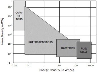
Figure 41. Ragone plot of power density versus energy density for different classes of energy storage/conversion systems, redrawn from [342]. Remarkably, supercapacitors bridge the gap between conventional dielectric capacitors on the one hand and batteries and fuel cells on the other.
Download figure:
Standard image High-resolution imageThe advantage of supercapacitors is in their ability to release large amounts of energy very rapidly. In electric vehicles, for instance, supercapacitors operating in parallel with batteries or fuel cells can provide considerable short-time power during acceleration or hill climbing [346].
For two decades, the development of supercapacitors has been an international endeavor involving scientists and companies in many countries. In Europe, relevant publications include, for instance, the following: [347–354] from France, [341, 355, 356] from Germany, [344, 346, 357–360] from Italy, [361, 362] from Poland and France, [363] from Switzerland, [364, 365] from the UK and [366] from Ukraine. For reviews see, for example those by Conway (Canada) [367], by Mastragostino et al (Italy) [346] and by Burke and Miller (USA) [368].
10.3. Mixed conduction and new materials
In figure 42, solid materials have been arranged according to their electric conductivities. These are usually perceived either as very small, as in typical insulators such as SiO2, or as ionic, as in the alkali and silver halides, or as electronic, as in metals and semiconductors, or as truly mixed as in silver sulfide. On closer analysis, however, it becomes evident that all ionic solids exhibit both ionic and electronic conduction. In fact, many chalcogenides and oxides, for example those with perovskite structures and compositions ABO3, are found to display substantial conductivities of either kind.
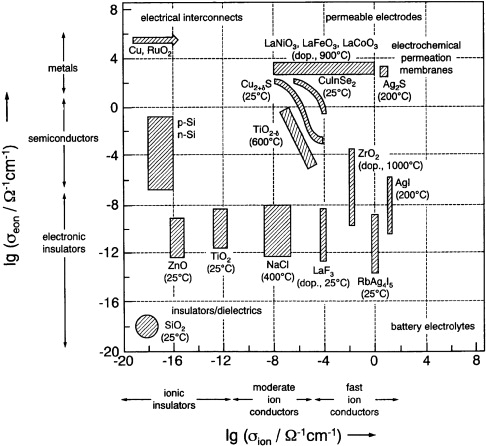
Figure 42. Double-logarithmic representation of electronic versus ionic conductivities of various solid materials. From [54], based on [372, 373].
Download figure:
Standard image High-resolution imageIn the early days of Solid State Ionics, it went without saying that ion-conducting materials with negligible electronic conductivities were most attractive. Later on, the importance of mixed conduction, in particular in electrodes, and also for applications such as in sensors and electrochromic devices, was increasingly appreciated. Much effort has since been put in finding new functional materials supporting mixed conduction and in optimizing their properties.
An interesting property of mixed conductors was discussed by Carl Wagner in 1956 [69]. A cell that is placed between two gaseous phases that differ in oxygen partial pressure will act as a permeation cell, allowing oxygen transport, as soon as not only oxygen ions but also electrons are mobile in the solid electrolyte. This is because, with the electrons being mobile, the requirement of electro-neutrality is easily fulfilled. Note that, in a steady-state condition, the gradients of the ionic and electronic electrochemical potentials are opposite to one another. Note also that, as a consequence of the validity of local electrochemical equilibrium, an e.m.f.-type voltage is built up across the sample. As might have been expected, its value differs from the one obtained by the usual Nernst equation by inclusion of the O2− transport coefficient [54, 69].
The selectivity of mixed-conducting oxides as permeation membranes, see the upper right corner of figure 42, can be exploited to separate O2 from other gases, which may be used for gas purification and chemical reaction engineering [54]. In this context, ten Elshof et al (The Netherlands) [369] suggested the perovskite-related mixed electrolyte Sr(Fe,Co)O3−δ as a relevant material. Other perovskites, which may also be used as oxygen-permeation membranes, were mentioned in a review written in 1997 by Bouwmeester and Burggraaf (The Netherlands) [370]. Much more recently, Belousov et al (Russia) [371] presented gas-tight ceramic composites consisting of ion-conducting δ-B2O3 and electronically conducting metal oxides such as In2O3 as ion transport membranes for oxygen separation from air.
Note, however, that a forced 'uphill' flow of mobile ions, either for 'electrochemical filtration' or for a deliberate regulation of partial pressures, requires application of a voltage for electrochemical pumping, as suggested in [332] and described in the previous subsection.
In view of the wealth of MIEC materials, methods, effects and applications, the readers' attention is drawn to two excellent reviews. One, written by Maier (Germany) [374] in 1984, is on the evaluation of electrochemical methods in solid state research, while the other, written by Riess (Israel) [375] in 1997, is a comprehensive treatment of the electrochemistry of mixed ionic/electronic conductors.
In the 1990s, fundamental aspects of transport in mixed ionic/electronic conductors were studied by the groups of Schmalzried (Germany) [376] and Janek (Germany) [377]. These concern the interference between ionic and electronic flows [376] and the influence of external forces such as, for instance, temperature gradients, which cause the Soret effect [377].
Every year, several conferences, review articles and books are devoted to new functional materials that bear relevance to Solid State Ionics. In view of this, the present text can only briefly indicate some of the most important lines of development, as seen from a European perspective.
Novel materials may be categorized in different ways. One is according to their ionic and electronic conductivities, as in figure 42. Other pertinent criteria are their historical origins on the one hand and their potential for applications on the other.
Remarkably, the history of many crystalline materials for Solid State Ionics can be traced back to Michael Faraday, Walther Nernst or Carl Tubandt. This includes the fluoride-ion-conducting compounds with the fluorite crystal structure, such as PbF2 (Faraday), the oxygen-ion-conducting fluorite-type materials, such as heterovalently doped ZrO2 (Nernst), and the structurally disordered solid electrolytes, such as the AgI-type solid electrolytes (Tubandt).
More recent members of the family of fluoride-ion conductors are CaF2, in which the number of fluoride vacancies may be enhanced by doping with LiF, as well as LaF3, where the same effect is achieved by doping with BaF2, see the detailed study by Roos et al (The Netherlands) [378].
As in YSZ, the high-temperature cubic fluorite structure of zirconia (cf figure 22) is also stabilized in solid solutions with other heterovalent oxides, while the number of mobile oxygen vacancies is at the same time significantly increased. In 1957, Kiukkola and Wagner [379] suggested to use CaO-doped zirconia in solid electrolyte cells in order to determine thermodynamic data of metal oxides.
In the early 1980s, different non-stoichiometric fluorite-structured oxygen conductors based on zirconia and ceria were experimentally and theoretically investigated by Kilner and Waters (UK) [380] and by Butler et al (UK) [381].
More recently, Martin (Germany) [382] presented a complete analytical model for the ionic conductivity of these materials. In a US–German collaboration, no experimental evidence could be found for fast diffusion along grain boundaries in YSZ, but oxygen transport rather seemed to be hindered by them [383]. In a joint project, Nakayama (Japan) and Martin (Germany) [384] studied the defect chemistry and oxygen-ion migration in doped ceria by first-principles density functional theory calculations. Subsequently, building on the results thus obtained, the authors and their German co-workers have been able to model the oxygen-ion conductivity in doped ceria, including its dependence on the fraction of dopant ions, by means of kinetic Monte Carlo simulations [385].
The group of crystalline fast ion conductors with structurally disordered sublattices is now no longer restricted to the AgI-type solid electrolytes and the β-aluminas, but has been considerably extended in the past decades, by the discovery of further families of solid electrolytes. These include the NASICON compounds, the pyrochlores and the so-called BIMEVOXes. In all these structures, the number of available sites by far exceeds the number of mobile ions, and the potential barriers between equivalent sites are favorably low.
NASICON, short for 'Na+ superionic conductor', was first synthesized by Goodenough et al [386]. This was done at MIT (USA), shortly before Goodenough became head of the Inorganic Chemistry Laboratory at Oxford University (UK). The composition of this synthetic material is given by Na1+xZr2P3−xSixO12, and the number of vacant sodium positions per formula unit is 3 − x. As reported by Kohler and Schulz (Germany) [387] the bottlenecks for sodium migration are widest for values of x around 2. By comparison with the β-aluminas, NASICON has the advantage of being a three-dimensional isotropic sodium ion conductor. It was, therefore, originally thought to be useful in replacing β-alumina in sodium/sulfur batteries for electrotraction. However, this has not materialized, because of two major disadvantages. (i) NASICON failed as an electrolyte as it was reducible by alkali metals. (ii) Similar to the β-aluminas, it was fragile and therefore hazardous to utilize in an electric vehicle. On the other hand, the material can be applied in sodium-selective electrodes and as thin-film material as suggested by Fabry et al (France) [388] and Morcrette et al (France) [389], respectively.
In 1980, Burggraaf and his co-workers (The Netherlands) studied Gd2O3–ZrO2 solid solutions and found a local maximum in the oxygen-ion conductivity at the pyrochlore composition of Gd2Zr2O7 [390]. Pyrochlores (such as Gd2Zr2O7) differ from fluorites such as YSZ by having a superstructure with twice the lattice parameter. Structural disorder is thus introduced by one out of eight oxygen positions being unoccupied, resulting in an oxygen-ion conductivity of about 0.001 Ω−1 cm−1 at 600 °C and of about 0.01 Ω−1 cm−1 at 900 °C, as measured in the case of Gd2Zr2O7 [390].
The first paper on Bi4V2O11 was published in France, by Abraham et al in 1988 [391]. The O2− ion conductivity of this compound was found to be as high as 0.01 Ω−1 cm−1 at 600 °C, thus exceeding the values of YSZ and the pyrochlores. Two years later, the same group discovered a new family of high-performance oxygen-ion conductors by substituting different cations for vanadium in Bi4V2O11 [392]. The materials thus obtained were called BIMEVOXes, with BI for bismuth, ME for the metal dopant, V for vanadium and OX for oxide. Unusually high conductivities were attained at relatively low temperatures, namely about 10−3 Ω−1 cm−1 at 300 °C. Measurement of the transport numbers indicated that those conductivities were almost exclusively ionic [392]. The defect chemistry of the BIMEVOXes has been discussed in great detail in a feature article written by Abrahams and Krok (UK and Poland) [393]. An impression of the significant disorder in the oxide sublattice is given by the Fourier map of figure 43, taken from [393].
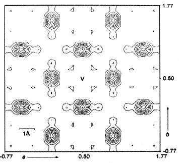
Figure 43. Fourier map generated from powder neutron diffraction data for quenched γ-BIMGVOX.10, Bi2Mg0.10V0.90O5.35−δ, showing diffuse scattering from oxide positions in the vanadate layer (section of a–b plane at z = 0), from [393]. Note that the time-averaged experiment does not distinguish between occupied and unoccupied sites.
Download figure:
Standard image High-resolution imageThe materials mentioned so far have been introduced above as members of the category 'historical origins'. For many others, including a variety of oxygen-ion, proton and lithium-ion conductors as well as MIECs and intercalation compounds, the category 'potential for applications' appears more appropriate. Accordingly, these will be referred to in those subsections, in which the advances made in the development of fuel cells and battery systems will be briefly outlined.
10.4. Interfaces and impedances
In polycrystalline materials, the transport of charge and matter is usually strongly influenced by grain boundary effects. With the help of microelectrode measurements, see e.g. Fouletier et al (France) [394] and, more recently, Fleig (Germany) [395], both highly conductive and highly resistive grain boundaries, occurring, for instance, in AgCl and in ceramic materials, respectively, are unequivocally detected and investigated [395].
In the following, let us consider ceramic materials with resistive grain boundaries. These were studied in the early 1980s by Burggraaf and co-workers (The Netherlands) [396, 397] and later by the group of Kleitz (France) [398]. For a simplified treatment, van Dijk and Burggraaf [396] introduced the so-called brick-layer model. This model has since been established as a reasonable approximation, see Maier and Fleig [399–401]. In particular, J Fleig could show that impedance spectra obtained by simulations on the basis of computer-generated microstructures, which contained irregular distributions of grain boundaries, reproduced experimental spectra very well and also did not markedly deviate from those derived from the brick-layer model [401]. Typical results as shown in figure 44 consist of two semi-circular arcs in the complex impedance plane.

Figure 44. Data in the complex impedance plane as obtained by a simulation technique which is based on computer-generated microstructures containing grain boundaries with different resistivities. Formally, the same pattern is generated by the equivalent circuit shown in the figure. From [401].
Download figure:
Standard image High-resolution imageOver the decades, the complex impedance,  , has become the most popular function for representing the electric and dielectric behavior not only of materials but also of entire electrochemical systems. For a review, see for example, Boukamp (The Netherlands) [402]. The most convenient plot is the one of - Z''(ν ) versus Z'(ν ), as in figure 44, in which the representative point traverses the arcs in a counter-clockwise sense, i.e. from right to left, as frequency is increased.
In the simplest case, when the available data are limited to frequencies below the onset of the frequency dependence of the bulk conductivity ('first universality') and neither grain boundary nor electrode effects are visible, the complex conductivity may be written as  , with both σ and ε being constant. In this case, the impedance, which is by definition proportional to the inverse of
  , becomes
  , with R denoting the dc resistance of the sample. This yields a semi-circle in the complex impedance plane, with Z'(0) = R , Z'(∞ ) = 0 and - Z''(ω ε0 ε /σ = 1) = R/2. A nice example of this behavior was measured in Maier's group on a single crystal of AgCl between two silver electrodes [403]. In figure 44, the respective semi-circle is the one on the left-hand side.
The low-frequency semi-circular arc, on the right-hand side, is due to the existence of the resistive grain boundaries, its size depending on their resistivity.
Phenomenologically, the two semi-circles are often described by the equivalent circuit shown in the figure. In terms of the dynamics of the mobile charge carriers, however, the low-frequency arc reflects the fact that their hopping motion is no longer random. When a grain boundary is encountered, this causes backward motion, which shows up in the velocity correlation function as a decaying negative component. Suppose this negative component decays as exp ( - t/τ ), then the complex conductivity is reduced by a term that is proportional to the Fourier transform of exp ( - t/τ ), i.e. to 1/(1 + iω τ ). With decreasing angular frequency, the real part, σ '(ω ), thus decreases according to σ '(ω ) = σ1 + (σ2 - σ1 )/(1 + ω2 τ2 ), from its bulk value, σ1, to its low-frequency value, σ2. The corresponding feature in the complex conductivity plane is a semi-circle and, when transformed into the complex impedance plane, becomes a semi-circle again, see figure 44. In terms of the parameters of the equivalent circuit of figure 44, the relaxation time introduced above is τ = R2 C2 R1 /(R1 + R2 ). This is the inverse angular frequency at the maximum of the conductivity arc. The respective maximum of the semi-circle in the impedance plane is, obviously, at 1/ω = R2 C2.
Note that a similar low-frequency arc, again reflecting an interfacial resistance phenomenon, will appear in the complex impedance plot, if the electrodes permit only a sluggish transfer of the mobile charge carriers [54]. In most practical cases, grain boundary and electrode effects are superimposed, and a separation of their contributions to the impedance data may be more or less straightforward.
Finally, let us consider a solid electrolyte between electrodes that perfectly block the passage of ions. Now the effects of electrode polarization completely dominate the dielectric behavior at low frequencies, when the ionic charge carriers are piled up or depleted at the electrodes. The resulting conductivity decreases rapidly with decreasing frequency, while the extra (relative) permittivity caused by the blocking, εB, increases tremendously, often attaining low-frequency values in excess of a hundred million [195, 404]. A simple model, which is based on the linearized Poisson–Boltzmann equation, has been repeatedly proposed in order to explain the roughly Lorentzian shape of εB (ω ) [405–407]. However, such a model treatment yields impossibly extreme ionic densities in the immediate vicinity of the electrodes and is, therefore, quite inadequate. The elementary error made is in treating the mobile ions like ideal-gas particles. In fact, the strong non-ideality of the piled-up or depleted ions necessitates replacement of the Boltzmann equation,  , by
, by  , where n(x)/n0 and a(x) are the normalized number density and the (unknown) position-dependent activity of the mobile ionic species, respectively [195].
10.5. Solid oxide fuel cells: kinetics and materials
The essentials for constructing solid oxide fuel cells were already known around the year 1900. By that time, Wilhelm Ostwald had shown that in a fuel cell chemical energy could be converted directly into electrical energy and that, importantly, the efficiency of the device was not limited by the maximum efficiency encountered in a thermodynamic process such as the Carnot cycle. Also, Walther Nernst had discovered heterovalently doped zirconia and identified it as an excellent 'conductor of the second kind'. Indeed, Nernst could have invented the solid oxide fuel cell himself, had he equipped his Nernst mass with suitable electrodes and had he placed it between air and a combustible gas at a temperature of about 1100 K. Moreover, he could have applied his Nernst equation to quantify the voltage of the cell, of course not including any overvoltage that would occur under current load.
The possibilities outlined above became quite evident, once Carl Wagner had explained the conduction mechanism in YSZ in 1943 [28]. However, it took four more decades until advances in ceramic technology rekindled interest in solid oxide fuel cells. This was pointed out by Steele (Imperial College, London) at the 6th International Conference on Solid State Ionics, SSI-6, held at Garmisch-Partenkirchen in 1987 [408]. Interestingly, the term 'solid oxide fuel cell (SOFC)' was not yet used in the title of his talk, but rather the expression 'solid state electrochemical reactor'. The even less widely known abbreviation 'SOFC' did, however, appear in the text of the Proceedings version of the paper [408]. Two years later, 'SOFC' had become so popular that Steele et al [409] included it in the title of their Hakone SSI-7 presentation.
In their publication [409], the authors reported on the 1980s development in the field, which had been dominated by the Westinghouse program and had led to the construction of a tubular array of a number of SOFCs in series, optimized to accept syngas fuels (mixtures of H2, CO and H2O) at about 1000 °C. Furthermore, based on oxygen exchange coefficients measured in 1984 by Kilner et al (London) [410], the authors made suggestions for mixed conducting oxide anodes for SOFCs that were designed for methane oxidation [409].
Within a few years, the continuing process of optimizing the components of SOFCs led to a particular choice, which is still popular at the present time. In their 1996 paper, Mogensen and Skaarup (Denmark) [411] described it as follows.
The oxygen-ion-conducting electrolyte was YSZ, typically containing about 8 mol% yttria. To keep ohmic losses low, the electrolyte layer was made as thin as technically feasible. The material chosen for the anode, i.e. the electrode at which the fuel flows toward the electrolyte, was a highly porous small-particle metal–ceramic mixture, for example Ni–YSZ. Such mixtures were dubbed 'cermets'. The cathode, however, at which elemental oxygen is reduced, was made of a mixed-conducting perovskite such as a strontium-doped lanthanum manganite, (La, Sr)MnO3−δ (LSM), or, rather, of an LSM–YSZ composite.
Notably, the use of perovskite-type oxides for SOFC cathodes dates back to pioneering work done at General Electric (USA) in 1969 [412].
In the present-day technology (2012), stacks of planar SOFCs, which are serially interconnected, are used as (mostly stationary) power units, often coupled with gas turbines. A well-suited interconnect material, LaCr1−xMgxO3, was already proposed in 1991, by van Dieten et al (The Netherlands) [413].
According to the 1996 paper by Mogensen and Skaarup, the rate-limiting processes at the electrodes were most probably taking place at the triple-phase boundaries. Therefore, to provide optimum reaction rates, not only porosities for gas diffusion but also long triple-phase boundaries were considered crucial [411]. Another study on the kinetics of porous mixed-conducting oxygen electrodes was published by Adler et al (UK) [414], also in 1996.
In the same year, Riess et al (Israel and Switzerland) [415] considered the I–V relations characterizing SOFCs and discussed in particular the potential drops at non-reversible electrodes.
Figure 45 is a sketch of the successive events occurring at the cathode of a SOFC, taken from a 1995 paper by Kreuer and Maier (Germany) [416].

Figure 45. Schematic diagram of events occurring in cathodes of SOFCs, from [416]. Note that the actual processes are usually much more complicated. Also, in contrast to reality, it has been assumed that oxygen is completely ionized when entering the electrolyte [54].
Download figure:
Standard image High-resolution imageIn the years to follow, further investigations aimed at separating and understanding the details of the electrode kinetics. Jørgensen and Mogensen (Denmark) [417], for instance, analyzed the impedance of LSM–YSZ composite cathodes and thus identified five different contributions, which they tentatively assigned to individual processes. Impedance measurements were performed also on Ni–YSZ anodes, by Primdahl and Mogensen (Denmark) [418], in order to identify and optimize the anodic rate-limiting steps. As a result, the fuel gas flow rate per unit of anode area was found to be decisive for the resistivity. The diffusion limitation was shown to be determined by the volume of stagnant gas outside the porous anode structure, rather than by the porous anode itself [419].
The dependence of electrode polarization resistances on geometric parameters was investigated by the group of Maier (Stuttgart, Germany). Their results highlighted the importance of lateral inhomogeneity and dimensional complexity as reflected by the respective contributions of bulk, surface and gas-phase diffusion [420].
In the past decade (2003–2012), a large body of work on the kinetics of reactions at SOFC cathodes has been completed at the Max Planck Institute for Solid State Research at Stuttgart, Germany [421–427]. In 2003, Fleig [421] reviewed efforts to reduce the electrode polarization resistance and presented results obtained from measurements with geometrically well-defined LSM cathodes. Thin-film microelectrodes were used in further work as well [422, 423], providing an excellent tool to circumvent the problems in detecting individual electrochemical processes, which are normally caused by the complex morphology of conventional porous electrodes. Besides LSM, the authors also used La1−xSrxCo1−yFeyO3−δ (LSCF) as thin-film microelectrode material upon single-crystalline YSZ [422]. A strong enhancement of the surface exchange kinetics was observed when lanthanum was replaced with barium, and (Ba, Sr)(Co, Fe)O3−δ (BSCF) was soon considered a prototype cathode material [423]. Measurement of the oxygen surface exchange kinetics on mixed conducting perovskites, covering compositions ranging from LSM to LSCF and BSCF, led to the conclusion that high oxygen vacancy concentrations as well as high vacancy mobilities in the perovskite are key factors for a high exchange rate [424, 425]. Theoretical predictions [426] were thus corroborated.
With regard to the more general question 'How is oxygen incorporated into oxides'? the reader is referred to a review by Merkle and Maier [427], which the authors dedicated to Hermann Schmalzried. Schmalzried's [428] own book Solid State Reactions gives an excellent introduction to the still much wider field of solid state kinetics.
During the last few years, essential properties of perovskite-type SOFC cathode materials have also been studied by the group of Sitte (Austria) [429–432]. These include their stabilities in different atmospheres, their non-stoichiometries, their oxygen exchange kinetics and their degradation in the presence of chromium.
A symmetric SOFC with (La, Sr)(Cr, Mn)O3±δ electrodes on either side of single-crystalline YSZ was recently built by a German/Italian group led by Janek (Germany). The authors observed a drastic dependence of the electrode kinetics on the absence or presence of a passivating SrO surface phase, which could however be removed by applying a cathodic potential [433].
Obviously, the most relevant functional materials for SOFC construction include strongly acceptor doped fluorite-type oxygen-ion conductors, such as YSZ, and perovskite-type conductors, such as LSM. Over the years, a number of investigations have aimed at a better understanding of oxygen transport in these solid electrolytes. Some of them, concerning YSZ and doped ceria, have already been mentioned in a previous subsection [382–385].
As early as in 1982, Kilner and Brook (UK) [434] published an experimental and theoretical study on the oxygen-ion conductivity in doped non-stoichiometric oxides. They considered in particular acceptor doped perovskite-type rare earth aluminates such as (La, Sr)AlO3−δ. For these materials they could show that (i) association commonly takes place between the dopant cations and the compensating oxygen vacancies and that (ii) the saddle point configuration for anion migration may be characterized by a critical radius, cf the broken circle in the right-hand panel of figure 46.
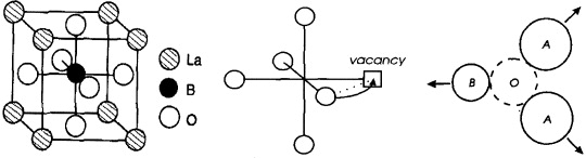
Figure 46. Left: cubic perovskite structure for a LaBO3 oxide. Center: curved path for oxygen-ion migration, along the edge of a BO6 octahedron. Right: saddle-point configuration for oxygen-ion migration, indicating cation relaxation. Here, A stands for lanthanum. From [435].
Download figure:
Standard image High-resolution imageIn 1995, Cherry et al (London) [435] applied computer simulation techniques to investigate the mechanistic features and energetics of oxygen diffusion in the cubic high-temperature phases of the perovskites LaBO3, where B stands for Cr, Mn, Fe or Co. Oxygen vacancies, created, for instance, by substituting Sr2+ for La3+, were thus shown to migrate along the edges of the BO6 octahedra, although not in a linear fashion, but via a curved path, which included the saddle point already described in [434], cf figure 46. Also, ion size effects were found to be important, with strontium fitting in best and, therefore, having the highest solubility on the lanthanum sublattice. A review of computer modeling results on ABO3 perovskites was given by Islam (UK) in 2000 [436].
Mogensen and his group (Denmark) studied the ionic conductivity of doped perovskites with composition (La, X)BO3−δ as a function of the choice of the cation B and the dopant X [437, 438]. The maximum oxide-ion conductivity, 0.14 Ω−1 cm−1 at 800 °C, was thus detected in the almost purely ionic conductor La0.8Sr0.2Ga0.8Mg0.2O2.8. Unlike doped LaGaO3, however, doped LaAlO3 and LaScO3 were found to be mixed conductors in oxidizing atmospheres. Notably, the degree of lattice distortion by the dopant was identified as the key parameter controlling the oxide-ion conductivity. Highest conductivities were attained, if the cubic lattice was kept as free of strains and distortions as possible, i.e. if Sr was chosen to replace La [438].
A broad overview of functional materials for solid state fuel cells was given in 2001 by Steele and Heinzel (UK and Germany) [439]. As pointed out by the authors, it had at that time become evident that there was a need for lowering the operating temperatures of SOFCs as far as possible, in particular for non-stationary applications. Indeed, intermediate temperature SOFCs (IT-SOFCs), operating not at 1000 °C but in the 500 °C to 700 °C temperature range, would provide many advantages, e.g. lower costs for materials and fabrication as well as a longer cell life. Various oxide-ion-conducting solid electrolytes have, therefore, been suggested as a replacement for YSZ, including acceptor doped ceria, the pyrochlores and the BIMEVOXes. Also, Islam and his group (UK) have drawn attention to oxygen transport in apatites [440, 441] and in structures containing tetrahedral moieties such as LaBaGaO4, [442].
Gadolinia-doped ceria, Ce1−yGdyO2−y/2 (CGO), usually with y = 0.1, was eventually selected as the optimum choice for IT-SOFC operation. An appraisal of this electrolyte was given by Steele (London) [443], on the basis of thermodynamic data and a bulk conductivity value of 0.01 Ω−1 cm−1 at 500 °C. Importantly, the oxygen-ion transport number was found to be close to unity in the IT-SOFC temperature regime [443]. In a frequently cited paper, Dusastre and Kilner (Imperial College, London) [444] identified porous composites of LSCF and CGO as matching cathodes. Shortly afterward, Kharton et al (Portugal) [445] published a review focusing on the compatibility of the CGO electrolyte and perovskite-type electrode materials such as LSCF. The broader field of transport properties of solid oxide electrolyte ceramics was reviewed in 2004 by Kharton et al (Portugal and UK) [446].
A further step in IT-SOFC cathode development consisted in the introduction of layered double perovskites such as GdBaCo2O5+δ and PrBaCo2O5+δ by Tarancón et al (Spain and UK) [447] and by Burriel et al (Spain and UK) [448], respectively. The oxygen surface exchange and oxygen tracer diffusion coefficients of these materials qualify them as excellent electrodes at temperatures between 500 °C and 700 °C. Ways to improve cathode/electrolyte interfaces have been proposed by Hildenbrand et al (The Netherlands) [449].
First results toward fabrication of micro solid oxide fuel cells (μSOFC) with nanocrystalline thin-film electrolytes and thin-film-based electrodes, as reported by Gauckler and his co-workers (Switzerland) [450], have lately attracted much attention.
For a recent review on functional materials for IT-SOFCs, the reader is referred to a publication by Molenda et al (Poland) [451].
The use of SOFCs can be seen not only in the generation of electric power but also in a high-yield co-generation of certain chemical oxidation products such as NO, the fuel being NH3 in this case [452]. Upon feeding both fuel and oxygen at the anode, Vayenas et al (Greece) [453] discovered the effect of electrochemical promotion of catalysis, also dubbed NEMCA (non-faradaic electrochemical modification of catalytic activity). The 'promoting' oxygen ions, migrating from the solid electrolyte to the catalytically active metal–gas interface, are obviously able to cause a pronounced and reversible alteration of the catalytic activation energy, rate and selectivity [454]. The process involves a change in the catalyst work function [454, 455]. For a more detailed explanation of the effect, see also [456] by Riess and Vayenas (Israel and Greece) and [457] by Fleig and Jamnik (Germany and Slovenia).
10.6. Proton exchange membrane fuel cells
In the first hydrogen/oxygen fuel cells, invented by C Schönbein and W R Grove in the late 1830s, the mobile hydrogen ions migrated from the anode to the cathode in a liquid electrolyte. In a proton exchange membrane fuel cell (PEMFC), however, the fuel gas, which may (but need not) be hydrogen, is separated from oxygen (or air) by a proton (but not electron) conducting membrane.
Proton conduction can be found in very different solid materials, from polymers to ceramics, and the operation temperatures of fuel cells in which they are employed as membranes are relatively low or relatively high, respectively. To distinguish between those two kinds of fuel cells, PEMFC is now normally used in the sense of polymer electrolyte membrane fuel cell, while PCFC stands for proton-conducting ceramic fuel cell.
In the late 1960s, W G Grot, who was born and educated in Germany and then joined DuPont in the United States, synthesized a hydrated perfluorosulfonic polymer called Nafion, which turned out to be highly proton conducting, electronically insulating and thermodynamically stable. For the chemical composition and microstructure of this 'acid sponge' [54] see the left-hand panel of figure 47.
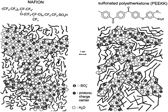
Figure 47. Schematic representation of the microstructures of Nafion and a sulfonated polyetherketone (from SAXS experiments), from [459].
Download figure:
Standard image High-resolution imageThin flexible membranes could be made of Nafion, making it perfectly suitable for fuel cells. Therefore, it soon became the polymer electrolyte of choice for PEMFCs. These were then used, for instance, in the NASA Gemini series of spacecraft. To cite from the 2001 review by Steele and Heinzel [439], 'Cells with high power density and very low degradation are already state of the art'.
However, this did not mean that there were no problems left. The following open questions were formulated by Steele and Heinzel [439] and, in the same year, also in an excellent review article written by Alberti and Casciola (Italy) [458].
- (i)Most probably, Nafion could not be widely used in fuel cells, e.g. for electrotraction, because of its inherently high cost in production. Were there less expensive alternatives?
- (ii)A similar question applied to platinum as a catalyst, not only because of its price, but also because of its limited availability.
- (iii)Could a PEM fuel cell be operated with a gas produced by reforming methanol or even gasoline? Could a reliable direct liquid methanol fuel cell be constructed?
- (iv)If so, how would the problems be avoided that were caused by the presence of CO at the anode, poisoning the Pt catalyst?
Scientists in many countries have tried to find satisfactory answers to these questions. Relevant 'European' answers are the following.
Low-cost alternative membrane materials for hydrogen fuel cell applications were suggested by Kreuer (Germany) in 1991 [459]. These were hydrated polymers based on sulfonated polyetherketones, denoted by PEEK or PEEKK. For the hydrated PEEKK material, the microstructure was determined by small-angle x-ray scattering (SAXS), see the right-hand panel of figure 47. As illustrated in the figure, the water-filled channels in the sulfonated polyetherketone are narrower, less separated and more branched than those in Nafion. For water volume fractions above around 25%, the proton mobility was found to be similar in both cases [459].
Regarding the CO poisoning of platinum as a catalyst, the thermolability of the adduct Pt–CO was an important piece of information. According to Alberti and Casciola [458], fuel cell working temperatures above 130 °C should drastically reduce or even eliminate the poisoning and even allow platinum to be replaced by more economical catalysts. Also, direct methanol fuel cells, efficiently working at temperatures between 140 °C and 160 °C, should be possible, with evident advantages when operating in cars [458].
In pursuit of working temperatures above the boiling point of water, the main idea has been to employ polymers with immobilized heterocycles as proton solvents [439, 459]. In their 2005 publication, Schuster et al (Germany) [460] could show that 1-heptylphosphonic acid does, indeed, combine good proton conductivity at 120 °C to 160 °C (even in the water-free state) with high thermo-oxidative and electrochemical stability.
Schuster et al [461, 462] were eventually able to report on the preparation of a novel polymeric proton conductor with exceptionally favorable properties. This electrolyte was a highly sulfonated poly(phenylene sulfone) with sulfone units ( ) connecting the phenyl rings, each of them being monosulfonated. While exhibiting excellent stability, this polymer electrolyte displayed a proton conductivity which, at temperatures between 120 °C and 160 °C and relative humidities between 15 and 50%, exceeded that of Nafion by a factor of five to seven [461, 462].
Certainly, these results have improved the prospects for PEMFC development considerably.
In the developing field of Solid State Ionics, protonic conduction in solids had been largely ignored before 1980, mostly because of the long absence of any good stable proton conductors. This was pointed out by Jensen (Denmark) and Kleitz (France) [463] in their preface to the volume 'Solid State Protonic Conductors I', which contained the Proceedings of a Danish–French Workshop held in Paris in December 1981. In September 1982, the Danish–French Workshop was followed by a European one on the same topic (SSPC II), now held in Denmark, with Goodenough (UK) joining Jensen and Kleitz in editing the Proceedings [464]. A series of workshops was thus started. It was later continued under the name of 'International Conferences on Solid State Protonic Conductors'. The Proceedings of the International Conferences have all been published in the journal Solid State Ionics, the most recent one (2012) being the 15th in the series.
Essential developments were outlined in the reviews published in the Proceedings, e.g. in those by Kreuer (Germany) [465, 466], Norby (Norway) [467] and Alberti and Casciola (Italy) [458]. One important aspect concerned the progress made in the preparation of perovskite-type oxides that exhibited at the same time high proton conductivity and good thermodynamic phase stability. For instance, covalent acceptor-doped BaZrO3 was identified as a proton conductor with potential for application as a ceramic membrane material in high-drain fuel cells operating at temperatures around 400 °C [466]. In a more recent paper, Haugsrud and Norby (Norway) [468] reported that Ca-doped LaNbO4 and chemically related perovskites were good proton conductors in wet atmospheres below 800 °C. The authors mentioned above [458, 465–467] also pointed out the use of solid state proton conductors in sensors and hydrogen pumps. As emphasized by Norby [467], there were important applications for solid state protonic–electronic conductors as well, for instance as hydrogen-permeable membranes in hydrogen separation technologies and as electrodes in high- and intermediate-temperature proton-conducting ceramic fuel cells.
For excellent comprehensive reviews of the state of the art in the science and technology of solid state proton conductors in the years 1992 and 2012, see the textbook by Colomban (France) [469] and the book edited by Knauth (France) and Di Vona (Italy) [470], respectively.
10.7. Lithium-ion batteries and beyond
First of all, the reader is asked to pardon the author for using the term 'battery' incorrectly in this subsection, i.e. not only for an array of galvanic cells but also for a single one. However, this has become the present-day common usage and must probably be considered an example of an ongoing etymological change.
Rechargeable ('secondary') batteries, operating at ambient temperature, have become part of our everyday lives. In fact, the advent of the lithium-ion battery, which is robust, lightweight and rechargeable, has revolutionized portable electronic devices such as mobile phones and lap-top computers. In electric and hybrid electric vehicles, up-scaled versions of it are now replacing batteries of the previous generation (mostly nickel metal-hydride).
More generally speaking, secondary battery systems have a crucial role to play in preserving our environment. If 'green' energy from wind or solar facilities is to be used, it is obvious that it is not normally generated when and where the consumer needs it. This necessitates not only off-peak power storage for load leveling but also off-grid power availability for portable devices and electrotraction. Energy must, therefore, be converted, stored and provided in a sustainable fashion. This is exactly what batteries are made for.
The lithium-ion battery owes its worldwide success mainly to two factors. One is the choice of the smallest and lightest metal ion, Li+, as the mobile charge carrier, resulting in high energy densities. The other is the use of both negative and positive intercalation electrodes, as in figure 48. Avoiding lithium metal as an anode (negative electrode) has the important consequence that explosion hazards due to dendritic lithium growth are thus kept at bay.
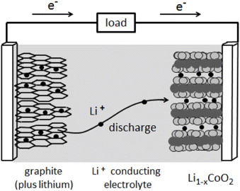
Figure 48. Schematic representation of a lithium-ion battery. The negative electrode (graphite) and the positive electrode (Li1−xCoO2) are separated by a non-aqueous liquid electrolyte. After [483].
Download figure:
Standard image High-resolution imageThe term 'intercalation' (or 'electro-insertion') refers to a host/guest solid state redox reaction [471]. In this reaction, electrochemical charge transfer is coupled with the insertion of mobile guest ions from the electrolyte into the structure of the solid host, which is a mixed electronic and ionic conductor. The expression 'intercalation' dates back to a paper published in 1971 by Rouxel et al (France) [472] on 'Les composites intercalaires NaxTiS2'. Substantial progress in the development of intercalation electrodes and in the understanding of the intercalation process itself could be made during the quarter century following the early 1970s, as summarized by Winter et al (Austria and Switzerland) [471] in their 1998 review.
Three years later, the most significant steps that had been taken at that time toward today's lithium-ion batteries were outlined by Tarascon and Armand (France) [473], in their review for Nature. Many of those steps had their origins in Europe, others in the USA and in Japan, see below.
The battery proposed in 1976 by Whittingham (USA) [310] had still made use of a metallic lithium anode. An important line of further development aimed at the prevention of the safety problems mentioned above. To this end, the reversible intercalation into graphite was extensively studied in the years to follow, in particular by Besenhard et al in Germany [474, 475] and by Basu et al in the USA [476, 477]. Basu's work led to the development of a workable intercalation electrode at Bell Labs.
A further major breakthrough was achieved in 1980, when Goodenough et al at Oxford University (UK) discovered that the layered intercalation compounds LiCoO2, LiNiO2 and LiMnO2 were excellent cathode materials [478]. Indeed, this family of compounds is still used in today's batteries.
The lithium-ion (or 'rocking chair') concept was suggested in 1980 by Armand in France [479] and by Lazzari and Scrosati in Italy [480]. However, it took about a decade for this concept to materialize. Most importantly, though, it triggered the development that led to the creation of the 〈graphite|liquid electrolyte|LiCoO2〉 battery in Japan [481, 482], which was then successfully commercialized by SONY in 1991. A schematic representation of it is given in figure 48.
The figure does not show the following details. The electrodes of the battery were (at least in the first generation) made of powders that contained millimeter-sized particles, and the non-aqueous liquid electrolyte was, in fact, trapped within the millimeter-sized pores of a polypropylene separator [483].
In its discharged state, the cell of figure 48 has negative and positive electrodes that consist of graphite and LiCoO2, respectively. Upon charging, Li+ ions are deintercalated from their LiCoO2 host, pass through the electrolyte and are then intercalated between the anodic graphite layers. The process is reversed upon discharging.
Since the introduction of this first-generation lithium-ion cell, substantial progress has been made concerning its three main components, i.e. the electrolyte as well as the negative and positive electrodes.
Regarding the electrolyte, efforts have aimed at replacing the non-aqueous liquid by a polymer of the PEO/lithium-salt type or even by a solid ion conductor. In 1992, for instance, the Bordeaux (France) group of Hagenmuller proposed a rocking-chair cell containing a lithium-ion-conducting polymer (see footnote 11), and in 1995 the Delft (The Netherlands) group of Schoonman reported on a rechargeable all-solid-state lithium battery using a ceramic BPO4:0.035Li2O electrolyte [484].
In the years to follow, many lithium-ion-conducting amorphous polymers were prepared and characterized, especially by Scrosati's group in Rome [485]. Yet, there were drawbacks in most cases, namely the necessity of cell operation at elevated temperatures and a lithium-ion transport number clearly below one [483]. An encouraging exception is PEO–LiBOB (BOB standing for bis(oxalato)borate). This polymer electrolyte, introduced by the Scrosati group in 2006, was explicitly made for application in low-temperature lithium rechargeable batteries [486].
The essential breakthrough was achieved when Bruce and his group at St Andrews (UK) discovered crystalline polymer electrolytes with excellent Li+-ion conductivities [273–276], cf the pertinent earlier subsection. Bruce and his co-workers reported also on the crucial effect of chain length on conductivity. This included an example in which a reduction from 44 EO units to 22 EO units caused an increase of the room-temperature conductivity of a crystalline polymer by three orders of magnitude [487].
A notable example of a non-polymer crystalline fast-lithium-ion conductor is Li7La3Zr2O12. A study of the structure and dynamics of this solid electrolyte was presented in 2011 by a group of scientists from six different institutions in Germany [488].
The most important features of a lithium-ion battery are, apart from its safety and cyclability, its energy density (in W h kg−1) and power density (in W kg−1). These quantities depend, respectively, on the number of Li+-ions that can be stored in the electrodes and on the rates of Li+-ion insertion and removal. While the guest ion/host ion number ratio is always limited to a maximum value around one, the rates of intercalation and de-intercalation can be increased significantly by reducing the characteristic diffusion lengths. In fact, the power densities of Li+-ion cells have been much enhanced by providing them with nano-particle or nano-structured electrodes, see e.g. Bruce (UK), Scrosati (Italy) and Tarascon (France) [483] as well as Jamnik (Slovenia) and Maier (Germany) [489].
At the negative electrode, replacement of the macroscopic graphite particles by nano-sized ones was found to have not only positive but also negative effects, especially with regard to safety. However, there are excellent alternatives.
One of them is the use of nano-wires made of the titanium oxide phase called TiO2-B, as described by the group of Bruce (UK) [490, 491]. The nano-sized diameter of these wires is suitable for fast lithium insertion and removal, while the few points of contact between individual wires, which are longer than 0.1 mm, ensure good electronic transport. In a British–Italian cooperation, these nano-wires were found to exhibit excellent performance when incorporated into lithium-ion cells [492].
A novel architecture negative electrode based on composites of TiO2 nano-tubes and iron oxide nano-wires has recently been proposed by a group of French and Spanish authors [493]. Generally, an advantage of nano-wires and nano-tubes is the availability of free volume for lithium insertion. Electrode volumes that change on intercalation and de-intercalation have indeed turned out to be a frequent problem, encountered, for instance, in LixMy alloys, see Winter and Besenhard (Austria) [494] and also Scrosati and co-workers (Italy) [495, 496].
Another viable solution for the negative electrode is the so-called displacement reaction, in which volume variations are largely buffered, as described by Tarascon et al (France) [497]. The authors started, for instance, with the alloy Ni3Sn4 and then used a first irreversible reaction with lithium to produce Ni and Li4.4Sn. On charging, Li4.4Sn was then decomposed into Sn plus 4.4 Li+ plus 4.4 e−, and on discharging this reaction was perfectly reversed. When the 'starting alloy', Ni3Sn4, was deposited on a nano-structured copper current collector, the structure consisting of isolated columns, the described procedure resulted in a high power density and excellent cyclability, with no change of the morphology [497–499]. We also note that, a few years earlier, a different displacement system for application in lithium cell anodes had already been proposed by Thomas (Sweden) [500].
Positive electrode materials for rechargeable lithium-ion batteries include lithium intercalation compounds such as LiCoO2, LiV6O13 and LiMn2O4 [471, 501].
The behavior of LiV6O13 as part of a composite positive electrode was first investigated by Steele et al (UK) in 1983 [502] and, in 1992, by the group of Thomas (Sweden), who performed a time-dependent in situ x-ray diffraction study of the phenomena occurring in it during cell discharge [503].
LiMn2O4 spinel has been known as an intercalation electrode material since 1983, when its suitability was first noticed by a British group of authors, including Goodenough and Bruce [504]. LiMn2O4 combines highest intrinsic rate capability with low cost and high safety and is, therefore, attractive as a cathode in lithium-ion cells for high-power battery units [505].
Since the turn of the millennium, LiFePO4 has been recognized as another most interesting cathode material. It was discovered in 1997 by the group of Goodenough, now at the University of Texas (USA) [506], who pointed out the role of the Fe3+/Fe2+ redox couple for lithium intercalation. In 2000, J O Thomas and his co-workers at Uppsala (Sweden) studied the processes of lithium extraction and insertion in LiFePO4 by x-ray diffraction and Mössbauer spectroscopy [507]. An atomic scale theoretical investigation of these processes was then published by Islam et al (UK) in 2005 [508], and the effects of partial substitution of Fe by Mn were investigated in 2006 by the groups of Molenda and Krok in Poland [509]. In 2001, the French group of Masquelier optimized LiFePO4/carbon composite electrodes [510], obtained e.g. by ball milling. Particle size reduction to the nanometer scale was shown to enhance electrode rate capabilities to levels of practical utility [511].
The present outline can only give a flavor of lithium-ion batteries. Therefore, most of the recent developments in theory, materials and battery design must remain unmentioned. A feature that deserves attention is, however, the so-called solid electrolyte interphase (SEI), sometimes also designated as solid electrolyte interface. An SEI is formed by the chemical reaction of a solid electrode (anode or cathode) with a liquid electrolyte, the more so the larger the contact areas are. Winter (Germany) has recently called it 'the most important and the least understood solid electrolyte in rechargeable lithium batteries' [512]. Basically, the SEI is formed by the reduction (oxidation) of the electrolyte at the anode (cathode). It consists of electrolyte decomposition products and forms a film allowing lithium-ion transport. At negative electrodes, the SEI layer has a mainly protective function, while its effect at positive electrodes may largely consist in causing a fading of charge storage. For a specific formation mechanism, see a further paper of Winter's group [513].
The most fascinating new advances in lithium batteries are probably those in developing rechargeable lithium-oxygen or lithium-air cells, as reported in 1996 by Abraham and Jiang (USA) [514] and more recently by the group of Bruce at St Andrews (UK) [515, 516]. As pointed out earlier, there is an inherent limitation to the energy density of lithium-ion batteries, i.e. to the quantity of lithium that can be stored in the intercalation electrodes. Theoretically, much higher energy densities might be attained if, at a suitably chosen porous electrode, lithium were allowed to react directly with O2 from the air, forming the peroxide, Li2O2, on discharging [515, 517]. On charging, the peroxide must then be decomposed again into lithium and oxygen. The main problem is to keep these processes sustainable for as many cycles as possible [516]. Surely, many challenges will still be met on the road to practical devices.
11. Concluding remarks
Solid State Ionics, as perceived today, is a grown and complex entity. Its structure bears resemblance to a big tree, with a strong trunk, several major branches and a multitude of smaller branches, leaves and blossoms that form its wide and beautiful crown. In this picture, a young scientist who decides to work in the field of Solid State Ionics may be compared with a bird, settling somewhere in the tree's outer parts. To this newcomer, the landing site and its immediate neighborhood will be familiar very soon, while the more distant sections of the crown as well as the trunk down below are not so easily seen.
The present author's goal has been to sketch the tree of Solid State Ionics as a whole and thus to provide the outlines of a map. This map is especially meant for newcomers to the field, with the purpose of giving them directions for exploring the marvels of Solid State Ionics themselves. The author's sketch has been made from his own vantage point, which is the European one. As already indicated in the introduction, the European perspective commands a unique view of the tree's trunk and major branches. However, to appreciate the beauty of its entire crown with its foliage and blossoms, the reader is asked to look at it from the viewpoints of the other continents as well.
It is also worth mentioning that the tree of Solid State Ionics keeps vigorously growing, with new research strategies and technological applications being implemented continuously. This is indeed required, if the pace of scientific development is to keep up with the needs of an increasing world population. Here, Europe is playing its part.
It goes without saying that the present review largely reflects the author's own perception of Solid State Ionics. This includes, for instance, the relative weights given to individual topics. Some of those who have actively contributed to the field may not find their work properly represented. Many important scientific results have not even been mentioned. Not unexpectedly, such deficiencies could not be avoided, and I apologize for them.
Acknowledgments
It is a pleasure to thank Malcolm Ingram and Joachim Maier for their generous help and advice. Also, I am grateful to my colleagues who sent me files of their papers. These include Michel Armand, Peter Bruce, Bernard Boukamp, Jürgen Fleig, Ludwig Gauckler, Saiful Islam, Janko Jamnik, Jürgen Janek, John Kilner, Philippe Knauth, Klaus-Dieter Kreuer, Franciszek Krok, Manfred Martin, Rotraut Merkle, Mogens Mogensen, Janina Molenda, Truls Norby, Ilan Riess, Werner Sitte, Josh Thomas, Costas Vayenas and Martin Winter.
Footnotes
- 1
From a soundtrack with Carl Wagner's own voice, by kind permission of Professor Tadashi Ohachi, Kyoto.
- 2
The acronym MIEC was probably first used by Ilan Riess, in his contributions to [55].
- 3
In this text, we stick to the notation for the phases of silver sulfide as introduced by Carl Tubandt, although this appears inconsistent now, in view of the existence of a further high-temperature phase, cf [56].
- 4
This function is
, i.e. the probability to find an ion at a given position at time t, if it was there at time 0. - 5
The Haven ratio, HR, is defined as D*/Dσ, where D* denotes the tracer diffusion coefficient, while Dσ = σkBT/(nq2) denotes the 'conductivity diffusion coefficient' as derived from the Nernst–Einstein relation.
- 6
van Gool in [307, p 373].
- 7
Huggins in [307, p 701].
- 8
Bruce in [308, p 87].
- 9
Steele in [307, p 103].
- 10
Armand in [307, p 665].
- 11
Delmas et al in [307, p 109].
- 12
Magistris in [308, p 213].
- 13
Lundén in [308, p 181].
- 14
Pizzini in [307, p 461].
- 15
Boukamp et al in [308, p 167].
- 16
Weppner in [308, p 9].
- 17
Fischer in [322, p 315].
