

Abstract
DI Hya is a short-period eclipsing binary and its classification has been discussed by several authors. New four-color light curves were obtained and have been analyzed together with the data from Manimanis & Niarchos simultaneously using the W–D method. The binary turns out to be a near-contact system where both components are filling or nearly filling their critical Roche lobes. The secondary has a temperature difference of ΔT ≃ −2800 K. The orbital period investigation has been ignored so far. All charge-coupled devices (CCD) and pe times of light minima are used for period analysis, showing that a cyclic variation with a short period of 1.46 years and a small semi-amplitude of 0.0034 days and a downward parabolic variation with a rate of  . The short period and small semi-amplitude cyclic variations were analyzed for the light-travel time effect via the presence of a close-in tertiary binary with an orbital separation shorter than 1.57(±0.31) au. Orbital properties of this close-in companion should provide valuable information on the formation of this short-period binary and stellar dynamical interaction. The downward parabolic change may be caused by angular momentum loss via an enhanced stellar wind of the more evolved secondary star.
Export citation and abstract BibTeX RIS

Original content from this work may be used under the terms of the Creative Commons Attribution 3.0 licence. Any further distribution of this work must maintain attribution to the author(s) and the title of the work, journal citation and DOI.
1. Introduction
The short-period (0.6147125 days) eclipsing binary DI Hya was first listed in Hoffmeister (1933) as a 203.1932 Hya name. After that, several authors gave its classification and some times of light minima. In the catalog of parameters for 1048 eclipsing binaries, Brancewicz & Dworak (1980) defined DI Hya as a semi-detached binary. Giuricin et al. (1983) examined the statistics of about 1000 categorized eclipsing binary systems, they obtained an uncertain contact (C ?) configuration for DI Hya. The binary was included in a list of near-contact binaries by Shaw (1994), who thought it is was possible subclasses of Algol (A ?). DI Hya (NSVS 15664134) was listed as known β Lyrae/Algol-type variables in Table 3 during the classification study of Hoffman et al. (2008). Isles (1988) gave visual observations of DI Hya, the secondary minimum was detected with the scattered light curve. The first BVRI light curves were presented by Manimanis & Niarchos (2007, hereafter MN), who analyzed the light curves with PHOEBE 0.28 program and the two best solutions in models 4 and 2 were obtained; however, the mass ratios of the two solutions had large differences. The model 4 solution was thought to be final one and was used for the following discussions in that paper because of its smaller rms χ2. They asserted that DI Hya is a near-contact binary only according to the relatively short distance between the two components, without calculating their fill factors. The orbital period investigation was ignored. DI Hya was observed in 2014 with the 1.0-m Cassegrain reflecting telescope at Yunnan Observatories (YNOs) in China to understand its configuration and evolutionary state and to investigate its orbital period changes.
2. New Multi-band Light Curves and Combined Photometric Solutions
The BVRI observations of DI Hya were carried out on 2014 January 2–4 and February 1 by using the PI 1024 TKB CCD photometric system attached to the 1.0-m Cassegrain reflecting telescope at YNOs. The CCD camera has an effective field of view 6 5 × 65. The integration times of each image for B, V, R, and I bands are 120 s, 60 s, 40 s, and 30 s, respectively. The same comparison star with MN was used. Using PHOT of the IRAF aperture photometry package, the observed images were reduced. The BVRI light curves plotted in Figure 1 were obtained from calculations of the phase of observations with the equation 2456662.28181+0
 61471231 × E obtained from the W–D results here. Eight times of light minima were obtained and are listed in Table 1 with our observations.
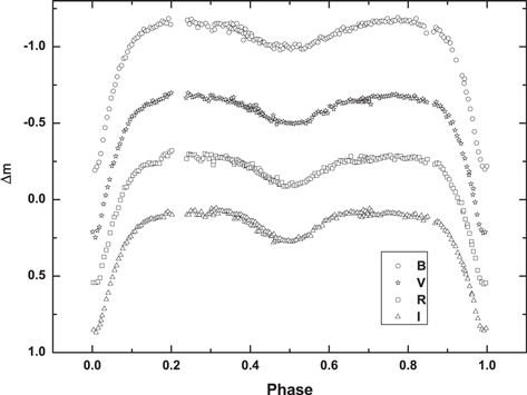
Figure 1. CCD photometric light curves of DI Hya in the BVRI bands obtained using the 1-m telescope at Yunnan Observatories in 2014. Open circles, stars, squares, and triangles refer to B, V, R, and I bands, respectively.
Download figure:
Standard image High-resolution imageTable 1. New CCD Times of Light Minima for DI Hya
| J. D. (Hel.) | Errors (days) | Min. | Filters |
|---|---|---|---|
| 2456662.28136 | 0.00018 | p | B |
| 2456662.28134 | 0.00026 | p | V |
| 2456662.28154 | 0.00027 | p | R |
| 2456662.28180 | 0.00023 | p | I |
| 2456690.25159 | 0.00053 | s | B |
| 2456690.25206 | 0.00046 | s | V |
| 2456690.25105 | 0.00085 | s | R |
| 2456690.25136 | 0.00099 | s | I |
Download table as: ASCIITypeset image
To understand the geometrical structure and evolutionary state of DI Hya, our BVRI data and the data from MN are analyzed together simultaneously using the W–D 2013 method (Van Hamme & Wilson 2007; Wilson 1979, 1990, 2008, 2012; Wilson & Devinney 1971 and Wilson et al. 2010) and yields one set of solutions that will reflect more reliable intrinsic features (such as mass ratio, inclination, temperatures, etc.) than if only one set of light curves is used.
Because no spectroscopic solution has been published, we adopted the following processing steps to derive a more reliable temperature of the primary star T1. The primary temperature was set to vary from 7000 to 9000 K with a step of 100 K according to an uncertain spectral type A6 for primary (Brancewicz & Dworak 1980), and the mass ratio was set to vary from 0.3 to 1.0 with a step of 0.1. Convergent solutions were achieved for each combination of temperature and mass ratio. Different models have been tried, and the solutions converged at models 2 (detached configuration) and 5 (semi-detached configuration with secondary fills its Roche lobe). The obtained relations between the resulting sum of the weighted square deviations Σ and mass ratio q are plotted in Figure 2, and the two models are used separately to find the best fit solution. As shown in the Figure 2, the smallest Σ values are achieved around T1 = 7300 K, q = 0.42 for model 2 and T1 = 7300 K, q = 0.39 for model 5, respectively. Therefore, the temperature of star 1 was fixed at T1 = 7300 K, the q was set to be adjustable at an initial value of q = 0.42 for model 2 and q = 0.39 for model 5, respectively. During the solution, the gravity-darkening coefficients g1 = 1.0, g2 = 0.32 and the bolometric albedo A1 = 1.0, A2 = 0.5 were chosen for two component stars. For the bolometric and bandpass limb-darkening coefficients, an internal computation with the logarithmic law was used. The final solutions were obtained by performing a series of differential corrections that are listed in Table 2. All theoretical light curves (solid lines) calculated with the solutions listed in Table 2 are plotted in Figure 3 with residuals (observed minus calculated light curves) from the solutions shown in the lower part. Figure 4 shows the geometrical structure of DI Hya at phases of 0.0, 0.25, 0.5, and 0.75, respectively. Model 2 shows a smaller  value compared with that of model 5, so parameters of model 2 were adopted for the following calculations. The determined mass ratio is about q = 0.4176, the inclination is about i = 88
 53, and the less massive component is nearly 2800 K cooler than the more massive one. The new ephemeris 2456662.28181+061471231 × E could be used for future calculations.

Figure 2. Relations between q and Σ determined by model 2 and model 5. Different color lines represent different primary temperatures.
Download figure:
Standard image High-resolution image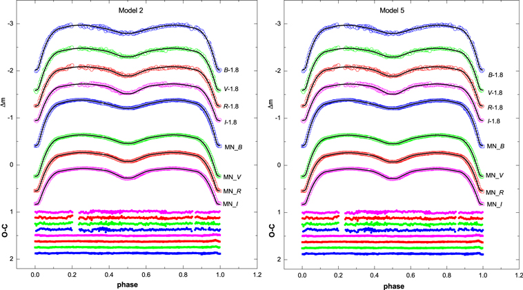
Figure 3. Observed (open symbols) and theoretical light curves (solid lines) obtained by solving the two sets of light curves simultaneously with models 2 and 5. Left panel for model 2, right panel for model 5. Residuals (observed minus calculated light curves) from the solutions are shown in the lower part of the figure.
Download figure:
Standard image High-resolution image
Figure 4. Geometrical structures of DI Hya at phases of 0.0, 0.25, 0.5 and 0.75, respectively.
Download figure:
Standard image High-resolution imageTable 2. Combined Photometric Parameters for DI Hya with Two Sets of Data
| Parameters | Model 2 | Model 5 |
|---|---|---|
| T1 (K) | 7300 | 7300 |
| T2 (K) | 4548 ± 21 | 4595 ± 12 |

|
88.53 ± 0.17 | 89.55 ± 0.01 |
q ( ) ) |
0.4176 ± 0.0064 | 0.3957 ± 0.0042 |

|
2.97548 ± 0.01107 | 2.94248 ± 0.00743 |

|
2.73613 ± 0.02174 | |
| HJD0 | 2456662.28181 ± 0.00008 | 2456662.28182 ± 0.00008 |
| P0 (days) | 0.61471231 ± 0.00000002 | 0.61471231 ± 0.00000002 |

|
0.3866 ± 0.0008 | 0.3886 ± 0.0014 |

|
0.4043 ± 0.0009 | 0.4064 ± 0.0018 |

|
0.4199 ± 0.0008 | 0.4213 ± 0.0033 |

|
0.2817 ± 0.0066 | 0.2817 ± 0.0008 |

|
0.2931 ± 0.0078 | 0.2937 ± 0.0009 |

|
0.3231 ± 0.0124 | 0.3263 ± 0.0009 |
| Our data: | ||

|
0.9501 ± 0.0050 | 0.9544 ± 0.0055 |

|
0.9181 ± 0.0062 | 0.9203 ± 0.0067 |

|
0.8850 ± 0.0104 | 0.8862 ± 0.0107 |

|
0.8473 ± 0.0164 | 0.8472 ± 0.0166 |
| Data from MN: | ||

|
0.9615 ± 0.0048 | 0.9656 ± 0.0055 |

|
0.9092 ± 0.0058 | 0.9113 ± 0.0061 |

|
0.8716 ± 0.0089 | 0.8726 ± 0.0092 |

|
0.8344 ± 0.0137 | 0.8341 ± 0.0138 |
| Our data: | ||

|
0.0260 ± 0.0051 | 0.0192 ± 0.0057 |

|
0.0351 ± 0.0065 | 0.0291 ± 0.0070 |

|
0.0466 ± 0.0112 | 0.0410 ± 0.0115 |

|
0.0632 ± 0.0178 | 0.0586 ± 0.0182 |
| Data from MN: | ||

|
0.0143 ± 0.0050 | 0.0077 ± 0.0056 |

|
0.0445 ± 0.0060 | 0.0385 ± 0.0064 |

|
0.0610 ± 0.0095 | 0.0558 ± 0.0098 |

|
0.0774 ± 0.0149 | 0.0731 ± 0.0151 |

|
0.00802 | 0.00824 |
Download table as: ASCIITypeset image
3. Variations of the O − C Diagram
Though DI Hya was discovered more than 80 years ago, the orbital period changes investigation has not been published. All the available 30 CCD/pe and 12 visual times of light minima are listed in Table 3. To fit the O − C curve satisfactorily, only CCD/pe data are used in our final analysis. (O − C)1 values are calculated with the new determined initial epoch and period. Weights of 1/σ2 were assigned to data, where σ is error of the times of light minima. By considering a general case (an eccentric orbit; e.g., Irwin 1952), the (O − C)1 diagram was described by the following equations:

Detailed explanations of each parameters were described in the paper of Liao & Qian (2010). It is clear from Equations (1) and (2) that we could determine six parameters (P3, T3, β, A,  , and e3) that fit the (O − C)1 curve. The fitting parameters from our analysis are listed in the upper part of Table 4. The fitting effect is displayed in the upper panel of Figure 5: the solid line shows a combination of a downward parabolic variation and a cyclic change, and the dashed line represents the downward parabolic variation that reveals a continuous decrease in the orbital period. The cyclic oscillation is analyzed for the light-travel time effect that arises from the gravitational influence of a possible third body. The parameters of the third body are estimated with the known equation

Figure 5. Cyclic variation constructed by CCD/pe data. The solid line in the upper panel shows a combination of a downward parabolic variation and a cyclic change,and the dashed line represents the downward parabolic variation that reveals a continuous decrease in the orbital period. The eccentric orbit of predicted close-in companion is more easily seen from the middle panel. Residuals from the whole effect are displayed in the lower panel.
Download figure:
Standard image High-resolution image
Table 3. Times of Light Minima of DI Hya
| JD (Hel.) | Method | Min. | Errors | E | Ref. |
|---|---|---|---|---|---|
| (cycle number) | |||||
| 2427503.3930 | vis | I | −47435 | (1) | |
| 2431173.2200 | vis | I | −41465 | (1) | |
| 2431176.3300 | vis | I | −41460 | (1) | |
| 2431178.1300 | vis | I | −41457 | (1) | |
| 2431181.2400 | vis | I | −41452 | (1) | |
| 2431194.1200 | vis | I | −41431 | (1) | |
| 2431197.1700 | vis | I | −41426 | (1) | |
| 2431208.2200 | vis | I | −41408 | (1) | |
| 2431221.1700 | vis | I | −41387 | (1) | |
| 2446114.4420 | vis | I | −17159 | (1) | |
| 2446135.3340 | vis | I | −17125 | (1) | |
| 2451276.1680 | CCD | I | −8762 | (1) | |
| 2451869.3690 | CCD | I | −7797 | (1) | |
| 2453432.5840 | CCD | I | −5254 | (1) | |
| 2453463.3199 | CCD | I | 0.0004 | −5204 | (2) |
| 2453757.45928 | CCD | II | 0.0008 | −4725 | (3) |
| 2453758.38132 | CCD | I | 0.0007 | −4724 | (3) |
| 2453857.9681 | pe | I | −4562 | (4) | |
| 2454058.9801 | CCD | I | 0.0001 | −4235 | (5) |
| 2454172.3965 | pe | II | 0.0003 | −4050 | (6) |
| 2454172.7022 | ccd | I | −4050 | (1) | |
| 2454212.6579 | ccd | I | −3985 | (1) | |
| 2454531.6923 | ccd | I | 0.0001 | −3466 | (7) |
| 2454535.3799 | pe | I | 0.0001 | −3460 | (8) |
| 2454816.3025 | CCD | I | −3003 | (9) | |
| 2454832.8990 | CCD | I | 0.0002 | −2976 | (10) |
| 2455257.6702 | CCD | I | 0.0001 | −2285 | (1) |
| 2455632.6470 | vis | I | −1675 | (11) | |
| 2455643.7061 | CCD | I | 0.0005 | −1657 | (12) |
| 2455933.8487 | CCD | I | 0.0005 | −1185 | (13) |
| 2454832.8983 | CCD | I | 0.0003 | −2976 | (14) |
| 2454882.6914 | CCD | I | 0.0002 | −2895 | (14) |
| 2455936.9206 | CCD | I | 0.0003 | −1180 | (15) |
| 2455986.7114 | CCD | I | 0.0002 | −1099 | (15) |
| 2456662.28136 | CCD | I | 0.00018 | 0 | The present paper |
| 2456662.28134 | CCD | I | 0.00026 | 0 | The present paper |
| 2456662.28154 | CCD | I | 0.00027 | 0 | The present paper |
| 2456662.28180 | CCD | I | 0.00023 | 0 | The present paper |
| 2456690.25159 | CCD | II | 0.00053 | 45.5 | The present paper |
| 2456690.25206 | CCD | II | 0.00046 | 45.5 | The present paper |
| 2456690.25105 | CCD | II | 0.00085 | 45.5 | The present paper |
| 2456690.25136 | CCD | II | 0.00099 | 45.5 | The present paper |
References. (1) O-C gateway: http://var2.astro.cz/ocgate/; (2) Hubscher et al. 2005; (3) Manimanis & Niarchos 2007; (4) Kazuo 2007; (5) Krajci 2007; (6) Hubscher 2007; (7) Samolyk 2008; (8) Hubscher et al. 2009; (9) Kazuo 2009; (10) Diethelm 2009; (11) Kazuo 2012; (12) Diethelm 2011; (13) Diethelm 2012; (14) Samolyk 2009; and (15) Samolyk 2013.
Download table as: ASCIITypeset image
Table 4. Orbital Parameters of the Close-in Companion
| Parameters | Values |
|---|---|
Revised epoch,  (days) (days) |
+0.00077(±0.00067) |
Revised period,  (days) (days) |
|
| Eccentricity, e3 | 0.56(±0.20) |
Long-term change of the orbital period, 
|

|
| Longitude of the periastron passage, ω3(deg) | 134(±17) |
| Periastron passage, T3(HJD) | 2455256.5(±26.2) |
| Light-travel time effect semi-amplitude, A (days) | 0.0034(±0.0005) |
| Orbital period, P3 (years) | 1.46(±0.01) |
Projected semimajor axis,  (AU) (AU) |
0.59(±0.09) |
| Mass function, f(m3) (M⊙) |

|
Projected masses,  (M⊙) (M⊙) |
1.01(±0.18) |
Orbital separation,  ( ( )(AU) )(AU) |
1.57 (± 0.31) |
Download table as: ASCIITypeset image
Based on the Simbad database4
, the color indices of DI Hya are calculated to be V–K = 0.63, J − H = 0.154, and H − K = 0.022, together with the temperature of primary star, suggesting a spectral type of about F0V (Cox 2000). Thus, the mass of the primary star is estimated as  (Cox 2000). According to the derived mass ratio of q = 0.4176, the mass of the secondary is
  . The parameter values estimated with the above equation are listed in the lower part of Table 4. It is shown that the eccentricity of the tertiary companion is
  ) and the mass function is
  . The mass of the third body is no less than 1.01(±0.18) M⊙ and the separation between the binary and the tertiary companion is shorter than 1.57 au. The eccentric orbit of predicted companion is more easily seen from the middle panel of Figure 5. Residuals from the whole fitting effect are displayed in the lower panel.
4. Discussions and Conclusions
The present combined photometric solutions suggest that both model 2 (for detached configuration) and model 5 (for semi-detached configuration with a secondary component) fills its Roche lobe and can solve the two sets of light curves simultaneously. These combined solutions are more reliable than if only one set of light curves is used. The present combined computation cannot converge at model 4 for a semi-detached configuration with primary fills its Roche lobe. MN used  K, but the combined solution value is 7300 K. The epoch and period are determined from the eight data sets. A larger value of i = 8853 and smaller value of q = 0.4176 are determined. Moreover, some problems exist in their analysis: (1) as one can see from the Figure 4 in their paper, the fitting of model 4 is not good; (2) the large difference between the mass ratios of their two solutions may suggest their analysis is uncertain; (3) if their mass ratio of q = 0.7066 is correct, the secondary component would estimated to be an F5V type star (Cox 2000), which does not accord with the fact of large temperature difference between the components (MN); and (4) according to their calculation, the secondary component evolves more than the primary one, which indicates the secondary component should first evolve to fill its Roche lobe, the model 4 is apparently not consistent with this status.
By using the formula ![${r}_{i}=\sqrt[3]{{r}_{i({pole})}\cdot {r}_{i({side})}\cdot {r}_{i({back})}}$](https://content.cld.iop.org/journals/1538-3873/129/973/034201/revision1/paspaa5869ieqn46.gif) and the well-known relation given by Eggleton (1983),
and the well-known relation given by Eggleton (1983),

the mean relative radius ri and Roche lobe radius RL can be calculated for the component stars. It reveals that in the case of detached configuration, the primary and secondary components are filling 88.5% and 97.3% of their critical Roche lobes, respectively, in the case of semi-detached configuration, the primary is filling 87.6% of its critical Roche lobe (f2 = 100%, secondary fills its Roche lobe for model 5). Two models yield similar parameters, the secondary has a temperature difference of ΔT ≃ −2800 K. As mentioned in Section 2, model 2 has a smaller  value, and therefore the binary is more likely to be a near-contact detached system where both components are filling or nearly filling their Roche lobes.
Based on all CCD and pe times of light minima, the first orbital period analysis is given. It is shown a cyclic variation with a short period of 1.46 years and a small semi-amplitude of 0.0034 days. The short period with small semi-amplitude cyclic variations are analyzed for the light-travel time effect via the presence of a close-in tertiary companion with an orbital separation shorter than 1.57(±0.31) au and a mass of  . This third body should be brighter than the secondary component of DI Hya and it would contribute light to the system. According to the relation of
  (Kippenhahn et al. 2012), the contribution of the third companion to the total system would then be roughly 16.7%. To check the presence of the third component, during the photometric solution we tried to add a third light (i.e., we made l3 an adjustable parameter). As listed in the lower part of Table 2, the third light is only about several percent. If this is true, as discussed by Liao et al. (2012) and Liao & Qian (2009), this low luminosity of the large mass third component may be explained that the third component might itself be a binary. Orbital properties of this close-in companion should provide valuable information on the formation of this short-period binary and stellar dynamical interaction.
Additionally, a downward parabolic variation with a rate of  is obtained in orbital period analysis. In common semi-detached Algol-type binaries with the secondary components fill their Roche lobes, orbital period present a trend of long-term increase changes, which could be caused by mass transfer from the secondary component to the primary one, e.g., TW Dra Liao et al. 2016). While the detected long-term period decrease of DI Hya should be caused by angular momentum loss (AML) via an enhanced stellar wind of the more evolved secondary star during its evolution (e.g., Tout & Eggleton 1988; Qian 2000, 2001; Qian et al. 2002; Wang & Zhu 2016).
This work is supported by the National Natural Science Foundation of China (nos. 11403095, 11325315, and U1631108), the Yunnan Natural Science Foundation (2014FB187), and the Strategic Priority Research Program "The Emergence of Cosmological Structures" of Chinese Academy of Sciences (grant no. XDB09010202).
Footnotes
- 4
http://simbad.u-strasbg.fr/simbad/, operated at CDS, Strasbourg, France.