

Abstract
Although extreme adaptive optics (ExAO) systems can greatly reduce the effects of atmospheric turbulence and deliver diffraction-limited images, our ability to observe faint objects such as extrasolar planets or debris disks at small angular separations is greatly limited by the presence of a speckle halo caused by imperfect wavefront corrections. These speckles change with a variety of timescales, from milliseconds to many hours, and various techniques have been developed to mitigate them during observations and during data reduction. Detection limits improve with increased speckle reduction, so an understanding of how speckles evolve (particularly at near-infrared wavelengths, which is where most adaptive optics science instruments operate) is of distinct interest. We used a SAPHIRA detector behind Subaru Telescope's SCExAO instrument to collect H-band images of the ExAO-corrected point-spread function (PSF) at a frame rate of 1.68 kHz. We analyzed these images using two techniques to measure the timescales over which the speckles evolved. In the first technique, we analyzed the images in a manner applicable to predicting performance of real-time speckle-nulling loops. We repeated this analysis using data from several nights to account for varying weather and AO conditions. In our second analysis, which follows the techniques employed by Milli et al. (2016) but using data with three orders of magnitude better temporal resolution, we identified a new regime of speckle behavior that occurs at timescales of milliseconds. It is not purely an instrument effect and likely is an atmospheric timescale filtered by the ExAO response. We also observed an exponential decay in the Pearson's correlation coefficients (which we employed to quantify the change in speckles) on timescales of seconds and a linear decay on timescales of minutes, which is in agreement with the behavior observed by Milli et al. For both of our analyses, we also collected similar data sets using SCExAO's internal light source to separate atmospheric effects from instrumental effects.
Export citation and abstract BibTeX RIS
1. Introduction
Extreme adaptive optics (ExAO) images consist of a point-spread function (PSF) core and a surrounding halo of speckles. The PSF core's size is determined by the diffraction limit of the telescope and the wavelength of observations, and the speckle halo has an angular size corresponding to that of the natural atmospheric seeing. The speckle halo is composed of speckles with intensities up to a few 10−3 times the intensity of the PSF core. Speckle causes include diffraction within the optical train and imperfect AO corrections due to time lag between wavefront sensing and correction, non-common path aberrations introduced between the wavefront sensor and science camera, and imperfect wavefront measurements due to noise. These speckles evolve on a variety of timescales, from hours (diffraction from the telescope spiders, for example) to millisecond (the deformable mirror's imperfect corrections for atmospheric turbulence) (Macintosh et al. 2005).
These speckles reduce the ability to detect faint features near a star such as extrasolar planets or debris disks, and their effect is orders of magnitude higher than photon noise. Racine et al. (1999) showed that the limiting brightness for detection is proportional to (1 − S)/S where S is the Strehl ratio, which emphasizes the need for ExAO instruments producing high Strehl corrections. The Strehl ratio is the comparison of the peak intensity of the measured PSF to the intensity of a PSF diffracted by the telescope pupil but otherwise unaberrated (Strehl 1902). The Strehl ratio will never be 100% for ground-based astronomical observations, so there will always be speckles, and several techniques have been developed to differentiate between them and actual structure in the science target. These include angular differential imaging (Marois et al. 2006) (which takes advantage of the rotation of the sky relative to an alt/az telescope) and spectral differential imaging (Smith 1987) (which utilizes the fact that the speckle halo expands with increasing wavelengths, but features in the target do not). However, because these techniques are implemented after the data have been collected, they do not remove the shot noise caused by the speckles. Additionally, because they are typically applied to long exposures, they have no effect on quickly-changing speckles. These techniques have been applied to obtain contrasts on the order of 10−6 at several tenths of an arcsecond from the PSF core. However, Earth-like planets in the habitable zones of M dwarfs have contrasts on the order of 10−7 to 10−8 (Guyon et al. 2012), and an Earth-like planet around a Sun-like star has a contrast of 10−10, so better speckle reduction strategies need to be implemented if such planets are to be detected.
Various techniques have been proposed for real-time speckle-nulling loops (e.g., Bordé & Traub 2006; Give'on et al. 2007; Sauvage et al. 2012; Guyon 2004; Baudoz et al. 2006; Serabyn et al. 2011). These provide two advantages over post facto speckle mitigation techniques such as those discussed above. First, they are able to reduce some of the dynamic speckles in addition to the static ones. However, the temporal bandwidths of the speckle-nulling loops that have been implemented on-sky have been relatively slow (Martinache et al. 2014), and these loops did nothing for speckles with lifetimes shorter than several seconds. A loop's temporal bandwidth determines to what extent the short-lived speckles can be reduced. The second advantage of real-time speckle-nulling loops is that, because they utilize interference principles to null the speckles, they remove the speckles' shot noise as well.
The lifetimes of speckles determine a given technique's ability to mitigate them, so several attempts have been made to define and measure speckle lifetimes. Vernin et al. (1991) was interested in speckle interferometry (a high-resolution technique that predates adaptive optics) and performed early speckle lifetime measurements. Macintosh et al. (2005) simulated speckle lifetimes in coronagraphic and noncoronagraphic data, and Stangalini et al. (2017) measured speckle lifetimes in AO-corrected visible-wavelength images using techniques more commonly applied to solar photospheric characterization. Milli et al. (2016) quantified the temporal changes in speckles by calculating Pearson's correlation coefficients (Pearson 1895) for frames separated by varying amounts of time. This analysis was most similar to ours; we describe their methods and results in Section 4.1. In this paper, we describe an experiment which utilizes high frame rate SAPHIRA speckle observations to identify the timescales over which speckles change and predict the contrast improvement that could be enabled by a real-time speckle-nulling loop.
2. Experimental Setup and Observations
The Subaru Coronagraphic Extreme Adaptive Optics instrument (Jovanovic et al. 2015b) (SCExAO) is an instrument at Subaru Telescope atop Maunakea in Hawaii. It utilizes a pyramid wavefront sensor and 2000-element deformable mirror (DM) updating at typically 2 kHz. AO188 (Minowa et al. 2010), Subaru's facility AO system, provides preliminary corrections, and then SCExAO provides high-order corrections to achieve Strehls of 80%–90% at H band (e.g., Kühn et al. 2018). SCExAO is designed to observe high-contrast objects such as extrasolar planets, brown dwarfs, and debris disks (Jovanovic et al. 2013, 2016). Numerous different modules can utilize SCExAO's corrected beam. Visible light is sent to the VAMPIRES (Norris et al. 2015) and FIRST (Huby et al. 2012) aperture-masking interferometers. Infrared light can be directed to the CHARIS integral field spectrograph (Groff et al. 2017), First Light Imaging C-RED 2 internal science camera (Gach et al. 2018), or the SAPHIRA camera.
SAPHIRA (Baker et al. 2016) is a 320 × 25624 μm pixel HgCdTe linear avalanche photodiode detector manufactured by Leonardo. It has low dark current (Atkinson et al. 2017) and noise and an adjustable gain, and it is optimized for high frame rates (up to 10 MHz per channel clocking frequencies). At bias voltages of ∼18 V, SAPHIRA detectors have a multiplication gain of several hundred (Atkinson et al. 2016). Because this gain multiplies the signal but not the read noise, SAPHIRA has the potential for photon-counting performance (Atkinson et al. 2018; Finger et al. 2016). SAPHIRA detectors can be read using 1, 4, 8, 16, or 32 outputs. Regardless of whether it is a full frame or subarray being read, the outputs read adjacent pixels. Therefore, unlike HAWAII detectors, all outputs are used even when reading a subarray, and the frame rate scales approximately inversely with the number of pixels being read (Goebel et al. 2018). We operated the SAPHIRA using a controller developed at the University of Hawaii Institute for Astronomy affectionately called the "Pizza Box" due to its shape. The persistence of modern SAPHIRA detectors is extremely low (even after saturating the detector by a factor of 10, no image remnants in later frames are visible), so it is not a concern for our speckle lifetime measurements.
During SCExAO engineering nights on UTC 2017 May 31, August 13, August 15, and September 11, we recorded SAPHIRA images of unresolved stars. These observations are summarized in Table 1. No coronagraph was used. The detector was subwindowed to 128 × 128 pixels (approximately 1.6'' per side) to achieve a frame rate of 1.68 kHz. During the first three nights, the PSF core was saturated by a factor of ∼10 to obtain a better S/N for the speckles; this data were used in the analysis of Section 3.2. On the night of September 11, most of the dynamic range of the detector was used, but the PSF core was not saturated; this data were used for the analysis of Section 4.2. On all nights, the SAPHIRA detector was operated in "read-reset" mode, wherein each line was read once and then reset. This enabled a maximum effective frame rate, optimal duty cycle, and full use of the dynamic range per image (Goebel et al. 2018). We later collected dark/bias frames and subtracted these to remove the detector's pedestal pixel-by-pixel offset pattern. In our previous speckle lifetime measurements (Goebel et al. 2016), we operated the detector in up-the-ramp mode (multiple reads followed by a reset) and then subtracted adjacent reads. This resulted in irregular time sampling and much poorer S/N due to having to split the flux over multiple reads. Additionally, in the previous observations, we used the PSF core to align the images in postprocessing, so we did not saturate it during observations. We have since developed other techniques as described below for tip/tilt correction in postprocessing. For these reasons, our more recent observations are much higher quality than the older ones.
Table 1. A summary of Observations
| UTC Date | Target | Seeing at 0.5 μm | Wind Speed | Strehl Ratio |
|---|---|---|---|---|
| (arcsec) | (m/s) | |||
| 2017 May 31 | Vega | 0.9 | 1.5 | 92% measured |
| 2017 August 13 | Altair | 0.35 | 2.5 | 70% estimated |
| 2017 August 15 | β And | Unreported | 2.7 | 90% measured |
| 2017 September 11 | 63 Cet | 0.35 | 0.7 | 90% estimated |
Note. The Strehl ratios were calculated from individual submillsecond exposures at H band collected with the SCExAO internal science camera, so they do not include the blurring effects of tip and tilt. The seeing measurements were produced by the Canada–France–Hawaii Telescope (CFHT) MASS/DIMM monitor, which is located approximately 750 m from Subaru Telescope. The wind speeds were recorded on the exterior of the Subaru dome. The May 31 data clearly had low wind effect PSF splitting (N'Diaye et al. 2018) visible, though this was not present in the images used for the Strehl ratio calculation. It was not obviously present in the August data, but the saturated PSF cores made it difficult to assess this. The September 11 data clearly did not have low wind effect present.
Download table as: ASCIITypeset image
The May and August nights produced the data used in the analysis presented in Section 3.2. On those nights, data sets were collected with SCExAO+AO188 (extreme adaptive optics) corrections, AO188 corrections only, and with no adaptive optics. In each regime, approximately one minute of data was collected with each of a 10 nm bandpass filter centered at 1550 nm, a 50 nm bandpass filter centered at 1550 nm, and a full H filter (about 260 nm bandpass). The narrower bandpass filters enabled better resolving of the speckles because they reduced the speckles' chromatic elongation. The three bandpasses in each of the three AO regimes produced nine data sets per night. To align images and provide a flux calibration, we applied an astrometric grid (Jovanovic et al. 2015a) during observations. In short, sine waves in orthogonal directions with frequencies optimized to the DM actuator pitch were applied to the DM. This generated an artificial speckle 15.5λ/D from the PSF core in each corner of the detector. By alternating the phase of the sine waves between 0 and π on timescales shorter than individual SAPHIRA exposures, the astrometric speckles became effectively incoherent with the speckle halo. This avoided coherent interference between the electric fields of the artificial and natural speckles that could distort the position and lifetime measurements. These astrometric speckles were 5.1 × 10⁻³ times the brightness of the PSF core for the May 31 observations and 2.6 × 10⁻³ the brightness of the PSF core during the August observations. We used these astrometric speckles to 1) align the images to remove tip/tilt, and 2) photometrically calibrate the speckle brightnesses.
The data from September 11 were used for the analysis presented in Section 4.2. We were interested in longer-term speckle evolution, so we collected seven minutes of ExAO-corrected PSF data. We again used the 50 nm bandwidth filter centered at 1550 nm; this bandwidth provided a good balance between throughput and chromatic speckle elongation. We did not use the astrometric speckle grid on this night; we aligned the images during processing by cross-correlating the speckle patterns from one image to the next.
SCExAO has an internal broadband light source and optics which simulate the telescope pupil (Jovanovic et al. 2015b). This produces a nearly-static PSF whose temporal evolution is solely due to instrumental effects. We observed this light source using the same camera settings as were used on-sky and then reduced the data using the same techniques as were employed for the on-sky observations. This enabled us to separate instrumental effects from actual atmospheric behavior. However, because this light source is internal to SCExAO, we were not able to probe the behavior of the telescope, image rotator, atmospheric dispersion corrector, or AO188 apart from the on-sky observations.
3. Speckle Lifetime Measurements for Real-time Speckle Nulling
3.1. The Benefits and Techniques of Real-time Speckle Nulling
Unlike speckles subtracted away during post-observation image processing, speckles interferometrically destroyed during observations do not leave behind photon noise. Because a speckle is fundamentally scattered starlight, it is possible to apply equal-amplitude but out-of-phase starlight on top of it and thereby destructively interfere it away. On the other hand, light from a substellar companion is not coherent with the starlight, so it cannot be destructively nulled away.
A number of techniques have been proposed to differentiate between speckles caused by scattered starlight and substellar companions and then mitigate the speckles. The pioneering work in real-time speckle-nulling algorithms and conceptually most straightforward method was proposed by Bordé & Traub (2006). The focal plane, which is where the science detector is located, shows the Fourier transform of the pupil plane, which is where the deformable mirror is located. A sine wave on the DM generates delta functions (PSFs) on the science detector. This is shown in Figure 1. The amplitude, phase, orientation, and frequency of the sine wave on the DM determines the brightness, phase, location, and spacing of the artificial speckles on the science detector. Therefore, one can generate an artificial speckle in the same location as an existing speckle, scan through phase space to find the opposite complex amplitude, and thereby null it away. The upside of this technique is that it is robust and does not require a detailed system model. The primary downside is that several phase measurements need to be made before a speckle can be nulled, so it is not as fast as other algorithms. Martinache et al. (2014) implemented this speckle-nulling algorithm on SCExAO. In practice, it worked well on the SCExAO internal light source for quasi-static speckles, but because the camera used operated at ∼170 Hz and was noisy, and the loop required many phase measurements per iteration, it was not fast enough to affect the dynamic speckles when tested on-sky.
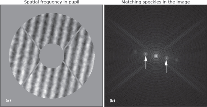
Figure 1. On the left is a map of deformable mirror displacement, and on the right are the resulting speckles produced in the focal plane. By varying the orientation, frequency, amplitude, and phase of the sine wave on the DM, one varies the location, spacing, brightness, and phase of the artificial speckles, respectively. Multiple sine waves can be applied to produce multiple speckles. Figure reproduced from Martinache et al. (2014).
Download figure:
Standard image High-resolution imageA more complex but potentially faster speckle-nulling method known as "electric field conjugation" (EFC) was proposed by Give'on et al. (2007). This method places small displacements on the deformable mirror to derive the electric field and thereby phase of speckles. It has produced the deepest contrasts (on the order of 10−9) in highly stable high-contrast imaging laboratories, but it requires a detailed system model and high S/N because the actuator pokes are quite small. The theory of this technique forms the basis of several other proposed speckle-nulling ideas. Other techniques for real-time speckle discrimination include coronagraphic focal plane wavefront estimator for exoplanet imaging (COFFEE; Sauvage et al. 2012; Herscovici-Schiller et al. 2018), the self-coherent camera (Baudoz et al. 2006), the phase-shifting interferometer (Serabyn et al. 2011; Bottom et al. 2017), synchronous interferometric speckle subtraction (Guyon 2004), and linear dark field control (Miller et al. 2017). However, apart from the implementation by Martinache et al. (2014) of the technique of Bordé & Traub (2006), none of these methods have been used for closed-loop speckle-nulling on-sky.9 This is primarily because they are optomechanically complex, require a higher degree of PSF stability than can be achieved on-sky, require very high Strehl ratios, or require deformable mirror perturbations that would be detrimental to science observations. Jovanovic et al. (2018) provides an informative review of these techniques.
Regardless of the particular algorithm, our speckle lifetime measurements are critical to quantify closed-loop speckle-nulling performance. As loop bandwidth increases, shorter-lived speckles can be destroyed, and therefore the focal plane contrast and detection limits improve. An understanding of the rates at which speckles change is important because it influences the feasibility of implementing the loops described above and gives the bandwidth necessary to reach a given performance level.
3.2. Our Observations and their Interpretation
Our goal is to measure how speckles evolve as a function of time and brightness. We quantified this using a new technique described below. The single largest detriment to image quality at SCExAO is tip/tilt caused by vibrations from the telescope and instrument (Lozi et al. 2016), which causes translation of the speckles instead of evolution, so it needed to be mitigated. Therefore, we began by aligning all the images. The results of the image alignment are shown in Figure 2. We located the artificial astrometric speckles and aligned images using those, and as a check also cross-correlated each image against the next to detect shifts. Both techniques registered images to ∼0.01 pixel accuracy and produced similar results.

Figure 2. Shown are three sample logarithmically scaled ExAO-corrected PSFs from the 2017 May 31 data set. The four bright speckles in the corners are the artificial astrometric speckles we created for image registration and photometry (the PSF core could not be used because it was saturated). Overplotted on the second and third images are circles indicating  and r = 10λ/D (the region within which we analyzed speckle lifetimes). The left image shows the result of coadding 10,000 frames (6 s of data), and the middle one shows the same coaddition after the images were aligned. Due to the alignment, the middle image exhibits many more airy rings and better-defined speckles than the left one. The right image is a sample individual frame. One astrometric speckle appears to be missing, due to a combination of a rolling shutter effect and the astrometric speckle modulation.
Download figure:
Standard image High-resolution imageSecond, we selected all pixels within a radius of 3λ/D <r < 10λ/D (0.12'' < r < 0.40'') of the PSF core. Given that the observed intensity I of a speckle is the square of the modulus of complex amplitude A,

it follows that

A is a random variable with a characteristic evolutionary timescale (temporal derivative). This is due to linearity between A and turbulence in the pupil, which to first degree, over adequately short timescales (a few ms), has a linear temporal evolution (fixed derivative). On these timescales, the temporal evolution of phase in the pupil is dominated by translation of turbulence layers due to wind. Because we are considering speckles at small angles (3–10λ/D), these correspond to low spatial frequencies on the pupil (period = 2.6–0.8 m). During a few milliseconds, a 10 m/s wind (which is higher than what we observed) translates a turbulence screen by a few cm. This is small relative to the aforementioned spatial frequencies in the pupil. For this reason, temporal evolution of phase can be linearized. There is linearity between phase in the pupil and complex amplitude in the focal plane, as the focal plane shows the Fourier transform of the pupil plane, and Fourier transforms are linear. Therefore, on millisecond timescales, the complex amplitude at the focal plane will evolve linearly.
For this reason, dA/dt is static over short timescales, and brighter (larger I) speckles will change more quickly than dimmer ones. Because of this, we sorted the pixels into four brightness bins (we selected the 20–30 percentile brightness pixels, 40–50 percentile, etc.). For each selection of pixels, we subtracted those pixels from the same pixels time t later. This formed a difference image. Finally, we calculated the standard deviation of these difference images to measure how the pixels changed in brightness over that time interval.10 If a pixel did not change in brightness, this quantity would be 0. We divided the standard deviation by the peak brightness of the PSF core so that it had units of contrast. We repeated this process for each image compared with 1–260 frames after it, and then averaged all the measurements at a given temporal separation to improve the S/N. We plotted this quantity against time for each brightness bin in Figure 3 (extreme AO, AO188 only, and no AO on the night of 2017 May 31) and 4 (extreme AO on 2017 August 13 and 15).
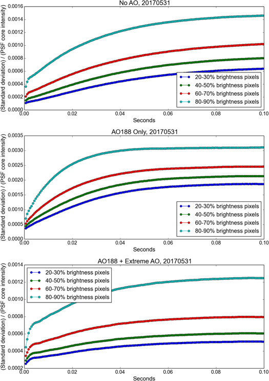
Figure 3. Shown here are the speckle evolution plots for four different brightness bins and the three different AO regimes (no AO, AO188 only, and AO188+ExAO) on the night of 2017 May 31. AO188 corrections reduced the standard deviation in speckle brightness relative to having no AO, and ExAO again reduced it relative to AO188. We divided the calculated standard deviations by the PSF core brightness to express them in units of contrast. It should be noted that the non-AO images were nowhere near diffraction-limited, so dividing the standard deviations by the peak brightness of the image resulted in misleadingly optimistic contrasts. The plots approach asymptotic values at large temporal separations because the speckles have entirely changed. The change in slope after a few ms in the ExAO plot is perhaps due to the linear approximation of complex amplitude breaking down. As predicted by Equation (2), the brighter speckles change more rapidly than the dimmer ones.
Download figure:
Standard image High-resolution imageTo understand whether the behavior of the standard deviations illustrated in Figures 3 and 4 was in fact due to speckle behavior or merely instrumental effects, we observed the SCExAO internal light source. There were no moving components in this setup. As is illustrated in Figure 5, indeed that speckle behavior is entirely static over the timescales examined. Second, we ran unilluminated frames through the above analysis pipeline to see how noise affected the plot's behavior. Again, the standard deviations were static in time. This means that the behavior in Figures 3 and 4 was indeed caused by the temporal evolution of the on-sky speckles.
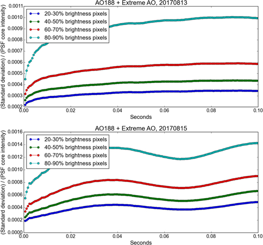
Figure 4. These two plots are equivalent to the bottom plot in Figure 3, but were produced using the extreme AO data collected on 2017 August 13 (top) and 15 (bottom). The seeing and AO tuning were significantly different in each of the three nights. The minor oscillation of the August 15 plot is likely due to a vibration that was not completely removed by our image alignment. We divided the calculated standard deviations by the PSF core brightness to express them in units of contrast. The change in slope after a few ms in the August 15 plot is perhaps due to the linear approximation of complex amplitude breaking down; it is unclear why this is not present in the August 13 data.
Download figure:
Standard image High-resolution image
Figure 5. To understand whether the behavior illustrated in Figures 3 and 4 was due to intrinsic atmospheric speckle evolution, we computed the standard deviations using images of the SCExAO internal light source and also dark frames collected immediately following the May 31 on-sky observations. The internal PSF data are reassuringly flat with time, indicating that the speckle evolution of the previous plots is not due to instrumental effects. A photometric calibration was not available for this data, so it is expressed in arbitrary brightness units. In the lower plot, the noise data are also flat with time. This has been scaled by the PSF brightness from the ExAO images collected a short time earlier to express it in units of contrast. The order of the relative brightnesses in this second plot is different from the other plots. This is most likely due to the behavior of pixels on the tails of the responsivity distribution; well-behaved pixels have the lowest standard deviations when unilluminated, and "bad" pixels are more prone to wandering and therefore higher standard deviations.
Download figure:
Standard image High-resolution imageIn all cases, the brighter speckles change in brightness more rapidly than the dimmer ones. This confirms the behavior we expected from Equation (2). The implication of this is that once a dark hole is present in an image, it is easier for a speckle-nulling loop to keep it dark. Because a dimmer speckle changes more slowly, more speckle-nulling loop iterations can be carried out before it changes. Therefore, the performance of a real-time speckle-nulling loop will be highly affected by the Strehl ratio and/or presence of a coronagraph that creates dark holes in the image.
On sufficiently short timescales, the complex amplitude can be approximated as behaving linearly with time, i.e.,

where a and b are the rates at which the real and imaginary parts of A change, respectively, and a0 and b0 are their initial values. Inserting this into Equation (1) and computing the measured intensity as a function of time I(t) produces

Therefore, the measured intensity of a speckle is a quadratic function of time, and its behavior depends on the complex amplitude's initial value and temporal rate of change. The standard deviation of pixel intensity, which is what we plotted in Figures 3–5, behaves the same way. For example, if a speckle is entirely static, then a = b = 0, and  , and this produces a flat line in the plot with a y-intercept which depends on the brightness the speckle. This exact case is illustrated in the top panel of Figure 5. On the other hand, the other simple case occurs when the speckles are changing (i.e.,
  and
and  ) but start from zero intensity (a0 = b0 = 0). In this case, the plot would exhibit an upward parabola centered at the origin. We approach this limit (but do not reach it) in the on-sky observations by selecting increasingly dim speckles (i.e., a0 → 0 and b0 → 0) for analysis.
Depending on the temporal sampling of the data, the initial brightness of the speckles, and the rates at which they change, this upward parabolic behavior may not be obvious in real-world measurements. The first few data points in the May 31 ExAO plot appear linear, the first few points in the August 13 plot appear downwardly parabolic, and only in the August 15 plot are the first few points plausibly upwardly parabolic. It is possible that our data are not fast enough to recover this predicted effect, and it would become apparent in data with even faster temporal sampling. The upward parabolic behavior assumes that the complex amplitude at a pixel changes linearly with time, and it certainly departs from this after a few milliseconds. Additionally, at sufficiently long timescales (≳0.04 s), the speckles have entirely changed from their initial state, causing the measured standard deviations to plateau. This is why our plots approach asymptotic standard deviations at large temporal separations.
If the behavior described by Equation (4) was evident in the images, one could predict the performance of real-time speckle-nulling loops from it. Because it is unclear whether our data reveal the predicted behavior, we will not do that, but we will explain how it could be done. If our analysis described above could be carried out at even higher temporal sampling or in an extremely high Strehl case, and the upward parabolic behavior revealed itself, one could fit a second-order polynomial to it. Solving this quadratic equation would provide the contrast that could be achieved at a given speckle-nulling loop bandwidth. The y-intercept in this fit would correspond to the read and photon noise (i.e., the noise that would be present if it was possible to image repeatedly with zero time between the images and with zero speckle evolution). A real-time speckle-nulling loop would zero the linear and constant terms with each update by forcing a0 = b0 = 0. In this case, I(t) ∝ t2. Therefore, the achievable contrast would increase with the square of the speckle-nulling loop bandwidth (where bandwidth is 1/t). This result emphasizes the major impact that speckle-nulling loops will have on detection limits.
4. A Different Approach: Extending the Analysis of Milli et al.
4.1. Milli et al.'s Technique and Results
Milli et al. (2016) employed a different technique for measuring the timescales over which speckles evolve. Their observations were comparable to ours, so we analyzed our comparatively higher frame rate data using their methods. They collected H-band images with a ∼55 nm bandpass at a frame rate of 1.6 Hz of coronagraphic PSF images from the SPHERE ExAO instrument. They then quantified the change in speckles over the 52 minutes of their on-sky observations by computing Pearson's correlation coefficient (Pearson 1895) for pairs of images. Pearson's correlation coefficient ρ(ti, tj) between two frames collected at times ti and tj can be defined as follows:
where the sum occurs over all pixels in the region S, I is the instantaneous intensity at a given pixel with position x,  is the instantaneous average intensity over the region, σ is the spatial standard deviation over the region, and Npix is the number of pixels in the region. The normalization is chosen so that ρ = 1 when ti = tj (equivalently, if the speckles did not change at all between images at ti and tj, ρ = 1). Milli et al. (2016) demonstrated that this quantity is directly related to the contrast obtained after subtracting one image of the pair from the other. The S/N of ρ for a single pair of frames is typically quite poor, so they improved it by averaging the values of ρ computed for many frame pairs separated by equal amounts of time.
After completing their on-sky observations, Milli et al. (2016) observed the instrument's internal light source and repeated the analysis to separate atmospheric effects from instrumental effects. In both cases, they observed two primary temporal regimes of speckle decorrelation. Over the first few seconds of their observations, the speckles decorrelated rapidly with an exponential decay. They fitted the first 30 seconds of their measurements with the equation

and found a best-fitting decay time of τ = 3.5 s for their on-sky observations. They initially posited that these speckles were primarily residuals of uncorrected atmospheric turbulence, but were surprised when then data collected using the internal light source exhibited the same behavior (in that case, they found τ = 6.3 s). They performed additional tests but were not able to identify the fundamental cause of this behavior, and in the end concluded that it was "real [and] related to an internal effect in the instrument independent of the atmospheric conditions or the telescope."
For images separated by greater than a minute, they observed a second regime of speckle change. They observed a linear decorrelation with time, and this was again present in both the on-sky data and also their internal lamp data. They suggested that this change in speckles must be caused by mechanical changes in the instrument (in particular the motion of the image derotator and thermal expansion effects). When they disabled the image rotator, this linear decorrelation of speckles became flat with time, i.e., the speckles were not measurably changing. In summary, they observed two regimes of speckle decorrelation, and these had different timescales for the on-sky and off-sky observations, but both were fundamentally caused by instrumental and not atmospheric effects.
4.2. Analysis of Our Data Using this Technique
Our data also consisted of H-band images of an ExAO-corrected PSF, but it had three orders of magnitude higher temporal resolution, enabling us to probe far shorter timescales. Additionally, because SCExAO is an entirely different instrument from SPHERE, we hoped our data might shed light on Milli et al. (2016)'s instrumental effects.
Our data had some important differences, however. First, the SPHERE data were collected behind a Lyot coronagraph, whereas our data were noncoronagraphic. Second, while their data were collected over 52 minutes, our data were 7 minutes in length, so we could not examine as long as timescales. We also recorded two 20-minute data sets of the SCExAO internal light source to differentiate between instrumental and atmospheric effects.
We then calculated Pearson's correlation coefficients according to Equation (5) using the annular region centered on the PSF and defined by radial separations 3λ/D <r < 10λ/D (0.12'' < r < 0.40''). Comparing each of the 630 thousand frames for the on-sky data and 1.99 million frames for the internal source data with each of the other frames in that data set would have been computationally prohibitive. Therefore, we compared each frame against 1, 2, 3, ..., 200, 208, 216, ..., 8400, 10080, 11760, ..., 604800 frames later. This enabled us to have maximum (S/N) at each calculated temporal separation, but we sacrificed temporal resolution at higher separations. In other words, we wanted the best time resolution at the shortest possible intervals, but settled for one Pearson's correlation coefficient data point every second at a time intervals greater than six seconds. This simplification reduced the computational load by 99.9%. Even after this, we calculated 852 million correlation coefficients for the on-sky data and 6.04 billion for the internal source data. The data points at a given temporal separation were then averaged to improve signal-to-noise. Because there are fewer frame pairs separated by large amounts of time, signal-to-noise decreased at larger separations. The on-sky data set was seven minutes long, and we calculated correlation coefficients for data points up to six minutes apart to still have reasonable S/N at the larger separations. The computation of the Pearson correlation coefficients for each plot took several CPU-days. Figures 6 and 7 show the results for the on-sky and internal light source data, respectively.
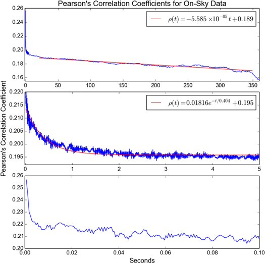
Figure 6. Plotted above are the Pearson's correlation coefficients calculated from seven minutes of SCExAO on-sky data. The same data are shown for three different timescales. Linear and exponential decays have been fitted to the data points between 20 and 350 s (top plot) and 0.1 and 5 s (middle plot), respectively. The coefficients of the fits are labeled. Unlike the plots of Section 3.2, less change in the speckles results in a higher value on the Y axis.
Download figure:
Standard image High-resolution imageWe observed three timescales of speckle evolution in the on-sky data. First, and most interestingly, our high frame rate data revealed an effect that Milli et al. (2016) did not observe. Frames separated by ≲2 ms are highly correlated in the on-sky data. After this time, the exponential decay behavior described in the next paragraph dominates. The minimal change in data points separated ≲2 ms is not present in the internal source data, implying that this is an actual atmospheric effect. This timescale is similar to the SCExAO loop bandwidth (2 kHz update rate, 15% gain, and 975 μs latency gives a 3 dB bandwidth of 240 Hz), so it is most likely explained by the changes to the deformable mirror shape. Over timescales of >2 ms, atmospheric speckles become decorrelated because they are corrected by the ExAO loop. Temporal correlations that naturally exist at >2 ms in the atmospheric speckles are erased or greatly attenuated by the ExAO correction; so there is a reduction in speckles with timescales of >2 ms.
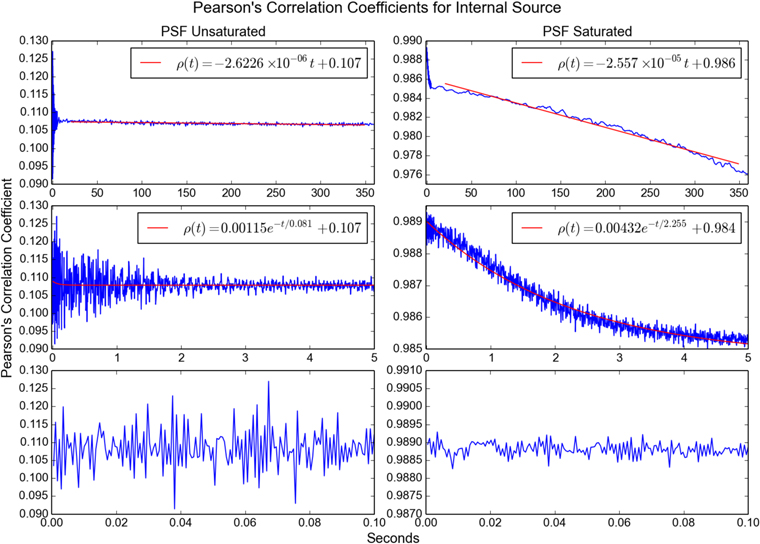
We recorded two 20-minute data sets using the SCExAO internal source. The first internal source data set had an unsaturated PSF core, mirroring our 2017 September 11 on-sky observations. However, because this was very nearly 100% Strehl (the slight degradation from 100% Strehl was due to imperfections in the optical elements of the instrument), very few speckles rose above the read noise of the detector. As a result, the calculation of the Pearson's correlation coefficients revealed no real speckle evolution (Figure 7 left plots). This mirrors the findings of Milli et al. (2016), who saw no speckle evolution when they froze the operation of SPHERE's optical elements. To improve signal-to-noise in the speckles, we then saturated the PSF core by a factor of 100 in the second internal source data set (Figure 7 right side). In this case, we observed two timescales of decorrelation as described in the following paragraphs. Although the PSF core of the on-sky data was unsaturated, we could measure speckle evolution there because the Strehl was lower (∼90% instead of ∼100%) and therefore the speckles were brighter.
Figure 7. Plotted above are the Pearson's correlation coefficients calculated from two 20-minute observations of the SCExAO internal light source. In the left plots, the PSF core was not saturated, mirroring our on-sky observations. However, because the PSF was nearly unaberrated, very few speckles were detectable, and no speckle evolution was measured. The dispersion in the correlation coefficients in these left plots is primarily caused by vibrations that were not perfectly removed by the image alignment process. On the right, the PSF has been saturated by a factor of 100, thereby improving the S/N of the speckles. In this case, timescales of speckle evolution are revealed. In each data set, the correlation coefficients are shown for three different timescales. Linear and exponential decays have been fitted to the data points between 20 and 350 s (top plots) and 0.1 and 5 s (middle plots). The coefficients of the fits are labeled. Note that the high correlation between frames separated by ≲2 ms of Figure 6 is not present in this data, indicating that it is an atmospheric and not instrumental effect.
Download figure:
Standard image High-resolution image
We observed a second timescale on the order of minutes over which the speckles linearly decorrelated in both the on-sky data and the saturated internal source data. We fitted a first-order polynomial to data points between 20 and 350 seconds and found that the speckles decorrelated by 56 parts per million (PPM) on-sky and 26 PPM on the saturated internal source over this period. For comparison, Milli et al. (2016) measured 25 PPM and 9 PPM for these two timescales, respectively, but their fit was performed over a different range of times. Because this decorrelation is present in both the on-sky and internal source observations, it is fundamentally caused by an instrumental effect. Unlike Milli et al. (2016), we did not use the image derotator; we had no moving components between the light source and our detector. This decorrelation must therefore be due to thermal expansions in the mechanics of SCExAO. This data depart from this linear decorrelation between 300 and 360 seconds in the on-sky data, but we think this is due to small number statistics (there are fewer frame pairs with 6 minute separations than, for example, 1 minute separations) than any intrinsic speckle behavior. The internal source data did not exhibit this effect.
The third timescale we observed was an exponential decay in the Pearson's correlation coefficients over the first few seconds for both the saturated internal source and the on-sky data. Milli et al. (2016) also observed this behavior, but in our case it occurred much more quickly. We fitted the points between 0.01 and 5 seconds with Equation (6) and found best-fitting parameters of τ = 0.40 s for the on-sky data and τ = 2.3 s for the saturated internal source. Our measured values for Λ and ρ0 are provided on the plots, but these have fewer physical implications because they are influenced by the flux level on the detector, as demonstrated by Figure 7. In contrast, Milli et al. (2016) found exponential decay terms of τ = 3.5 s and τ = 6.3 s for their on-sky and internal light source data, respectively, when fitted to timescales between 1 and 30 seconds.11 We observed a much more rapid decay than them, but the exponential decay behavior was present in both observations. Milli et al. (2016) were unable to explain the cause of this effect.
Whereas the analysis presented in Section 3.2 had applications to real-time speckle nulling, the results presented here are primarily applicable to speckle reduction during postprocessing. If the exposure times of individual images in an observing sequence are shorter than the timescales on which speckles evolve, then postprocessing techniques such as KLIP (Soummer et al. 2012) and LOCI (Lafrenière et al. 2007) will be better able to subtract the speckles. For this reason, it is advantageous to use short exposures while conducting observations for which the speckle halo is relevant (this must be balanced against the read noise of the detector, emphasizing the need for low-noise detectors such as SAPHIRA or electron-multiplying CCDs). Although it is preferable to have the speckles as dim as possible, as these have minimal photon noise, it is also ideal for the speckles that still exist to evolve as slowly as possible, because this enables them to be mitigated during data reduction. This emphasizes the need to have the instrument maximally mechanically and thermally stable. Indeed, SPHERE has more thorough environmental/thermal stabilization than SCExAO, which likely explains why the speckle decorrelations measured in this section occur more rapidly than those of Milli et al. (2016).
5. Conclusions
We collected H-band images of the speckle halo surrounding the SCExAO PSF at a frame rate of 1.68 kHz. We then analyzed the data to see how speckles evolved as a function of time and brightness. We performed two analyses: we used a new technique to quantify speckle lifetimes with implications to real-time speckle-nulling loops, and we performed a second analysis with more general applications following the standard techniques in the literature. Our data used in the second analysis had three orders of magnitude higher temporal resolution than that used for previously published studies, and we identified a new timescale of speckle decorrelation. We observed that speckles were relatively static for timescales of ≲2 ms in on-sky data, and we suggest that this timescale corresponds to the bandwidth of the ExAO loop. For timescales on the order of seconds and minutes, we observe similar behavior to that identified by Milli et al. (2016), namely an exponential decay over the first several seconds, followed by a linear decay over minutes. Mirroring the results of Milli et al. (2016), these two trends were present in both the on-sky and internal source observations. They noted that the linear decorrelation over minutes went away when the image rotator was stopped, but we observed this effect even without an image rotator.
An understanding of the timescales over which speckles evolve can inform the development and deployment of speckle mitigation techniques. A higher bandwidth speckle-nulling loop can destroy a greater fraction of speckles and thereby enable the detection of higher-contrast substellar companions. For about 300 nearby M dwarfs, the angular separation of an Earth-like planet in the habitable zone at maximum orbital elongation would be at least 1 λ/D in the NIR for a 30-m-class telescope (Guyon et al. 2012), and the contrasts of these targets are in the range of 10−7–10−8. Although current techniques struggle to produce processed contrasts better than 10−6 at much larger angular separations, ELTs and the implementation of improved speckle reduction techniques, both during observations and during data processing, will enable observation of these targets.
The authors acknowledge support from NSF award AST 1106391, NASA Roses APRA award NNX 13AC14G, and the JSPS (Grant-in-Aid for Research #23340051, #26220704, and #23103002). This work was supported by the Astrobiology Center (ABC) of the National Institutes of Natural Sciences, Japan and the director's contingency fund at Subaru Telescope. F.M. acknowledges ERC award CoG 683029. The authors recognize the very significant cultural role and reverence that the summit of Maunakea has always had within the indigenous Hawaiian community. We are most fortunate to have the opportunity to conduct observations from this mountain.
Footnotes
- 9
It is worth noting that Kasper et al. (poster presented at In the Spirit of Lyot 2015 and obtained through private communication) used EFC to create a dark hole on the SPHERE internal source and then applied this static map on-sky.
- 10
Because some pixels will become brighter and other pixels will become dimmer from one image to the next, it makes more sense to calculate a standard deviation than a mean or median, as these latter two quantities would on average be zero.
- 11
We performed the fits over a different range of times than Milli et al. (2016) because in the case of the linear decay, we simply did not have long enough time coverage, and in the case of the exponential decay, the fit would have been poor if we fitted to the same 1–30 s range as them.