


ABSTRACT
Using the Sloan Digital Sky Survey (SDSS), ∼900 deg2 of the sky surrounding M31 and M33 have been searched for globular clusters (GCs) that through galaxy interaction have become unbound from their parent systems and M31 (hence, intergalactic globular clusters, IGCs). This search reached a maximum of ∼500 kpc in projected galactocentric distance (Rgc) from M31. Visual examination of 283,871 SDSS cutout images and of 1143 fits images yielded 320 candidates. This sample was reduced to six GCs and one likely candidate by excluding galaxies on the basis of combinations of their optical, ultraviolet, and infrared colors from the SDSS, the Galaxy Evolution Explorer satellite, and the Wide-field Infrared Survey Explorer satellite, as well as their photometric redshifts from the SDSS. Since these seven objects have 14 kpc ⩽ Rgc ⩽ 137 kpc, they are more likely to be GCs in the halo of M31 than IGCs. They are all "classical" as opposed to "extended" GCs, and they provide further evidence that the remote halo of M31 (Rgc ⩾ 50 kpc) contains more GCs of all types and, in particular, far more "classical" ones than the remote halo of the Milky Way.
Export citation and abstract BibTeX RIS
1. INTRODUCTION
Intergalactic globular clusters (IGCs) are globular clusters (GCs) that are not bound to individual galaxies, but are instead moving in the potential of a galaxy cluster or group. They have been found in the Coma (Peng et al. 2011), Virgo (Lee et al. 2010), A1185 (West et al. 2011), and A1689 (Alamo-Martínez et al. 2013) clusters of galaxies. The simulations by Bekki & Yahagi (2006) suggest that IGCs are produced by tidal stripping during galaxy–galaxy interactions, are concentrated at the centers of the galaxy clusters, and may exist in galaxy groups as well as clusters. The globular cluster GC-2 in the M81 group, which is ∼400 kpc from M81 according to the distance measured by Jang et al. (2012), may be an IGC in a galaxy group. At one time, the Milky Way (MW) GCs lying at galactocentric distances ≳ 100 kpc were considered IGCs, e.g., Pal 3 and 4 (Burbidge & Sandage 1958), but now they are thought to be bound to the MW (e.g., Wilkinson & Evans 1999). The possibility that IGCs may exist in the Local Group has motivated this search for GCs at large distances from M31, which must be the best location to look for them.
Several observations suggest that galaxy–galaxy interactions have been more frequent in the environs of M31 than near the MW. M32, the very compact elliptical companion of M31, may be a tidally stripped galaxy (Faber 1973) or the product of a galaxy merger (e.g., Kormendy et al. 2009). Recent surveys of M31 have revealed that it has a giant stellar stream (GSS) and other stellar overdensities in its halo, which are probably the debris from galaxy accretion events (e.g., Ibata et al. 2001; McConnachie et al. 2009). The model of Fardal et al. (2013), for example, suggests that the GSS, which spans ∼150 kpc, is the relic of the tidal destruction of a galaxy about the size of the Large Magellanic Cloud. With the discoveries of the Sagittarius dwarf spheroidal (dSph) galaxy and its tidal streams and of other stellar overdensities in the MW's halo, there is no question that the MW has accreted satellite galaxies. None of the known overdensities in the MW's halo are, however, on the scale of the GSS. The recent surveys of M31 have also identified a large number of satellite galaxies, and over the same range in luminosity, M31 has ∼2 times the number of satellites as the MW (Yniguez et al. 2014). It has been known for decades that M31 has a much larger population of GCs than the MW, and this disparity has been growing in recent years as M31 has been more thoroughly searched. The total number of MW GCs is now 157 (Harris 1996, 2010 edition), and the few additions over the last decade are either heavily obscured clusters that lie near the Galactic plane or center or very low-luminosity clusters. There are 638 confirmed GCs in version 5 of the Revised Bologna Catalog of M31 globular clusters and candidates (RBCv5; Galleti et al. 2004, 2012 edition), and additional GCs and candidates have been identified more recently (di Tullio Zinn & Zinn 2013; Mackey et al. 2013). The ∼4 times larger population of GCs in M31 is not solely a consequence of its larger bulge because about the same factor is found if the GC populations are compared at, for example, galactocentric distances greater than 40 kpc. If the GCs in the outer halos of spiral galaxies were accreted from tidally disrupted satellite galaxies (e.g., Searle & Zinn 1978), which is strongly supported by the evidence that several MW GCs were once members of the Sgr dSph galaxy (see review by Law & Majewski 2010) and by the association of some M31 GCs with its halo overdensities (Mackey et al. 2013; Veljanoski et al. 2013), then the larger number of remote GCs in M31 than in the MW may be a consequence of M31's larger population of satellites and its apparently richer history of satellite accretions.
While there is no direct evidence yet, some of the galaxy–galaxy interactions involving M31 and its satellites, and/or between satellites, may have produced IGC's. In this paper, we describe our search for IGCs and for GCs in the remote halo of M31, which has used a combination of visual inspection of images and optical, infrared (IR), and ultraviolet (UV) photometry.
2. THE SEARCH AREA
Following the methodology of di Tullio Zinn & Zinn (2013, hereafter Paper I), our selection of GC candidates is based on the photometry in data release 8 (DR8) (Aihara et al. 2011) of the Sloan Digital Sky Survey (SDSS). Unfortunately, the SDSS footprint does not cover uniformly the sky around M31, which limited the extent of our survey and produced its odd geometry. Figure 1 shows the regions of the sky that we have searched in this paper and in Paper I. The current search covered ∼900 deg2, and reached a maximum of ∼500 kpc in projected galactocentric distance (Rgc) from M31, assuming its distance is 780 kpc (McConnachie et al. 2005). Most of the area of the survey has 130 kpc ≲ Rgc ≲ 390 kpc. For comparison, the dSph galaxy farthest from M31 in Figure 1, Andromeda XXVIII, has Rgc ∼ 365 kpc.

Figure 1. In this map of the sky, the large plusses mark the positions of M31 and M33. The crosses mark the positions of the dwarf elliptical galaxies NGC 147 and 185, and the asterisks mark the locations of the dSph satellite galaxies of M31. The solid lines are the borders of the regions where GCs were searched for in this paper. The dashed lines are the borders of the regions searched in Paper I. The odd shapes of these regions are due to the footprint of the SDSS survey in this region of the sky.
Download figure:
Standard image High-resolution image3. SEARCH CRITERIA
3.1. Candidate Selection
Our candidate GCs were selected from the objects classified as non-stellar by the SDSS. Following the procedures of Paper I, we used the interstellar extinctions and the magnitudes in the SDSS galaxy catalog to select objects that have 0.3 ⩽ (g − i)0 ⩽ 1.5 and 14 < r0 < 19.0. This range in color encompasses the range of the old M31 GCs (Peacock et al. 2011; Kang et al. 2012) and also the range in color of Maraston's models (Maraston 1998, 2005)1 for stellar populations of one age and one chemical composition (simple stellar populations, SSPs) that have ages from 1 to 15 Gyr and metallicities from 0.005 to 3.5 solar. The magnitude range includes approximately the brightest 5 mag of the luminosity function of the GCs in M31 (−10.5 ≲ Mr ≲ −5.5, if 780 kpc is adopted for M31's distance, McConnachie et al. 2005). According to Maraston's SSP models, the corresponding range in mass is ∼4 × 10⁶ to 4 × 10⁴ M☉. In Paper I, we used the Petrosian magnitudes that are listed in the SDSS galaxy catalog. Here we use instead the "model magnitudes" because they have slightly smaller errors than the Petrosian magnitudes at the faintest magnitudes that we are considering (i.e., r ∼ 19).
3.2. Visual Inspection
The outer halo of M31 contains both "classical" and "extended" GCs in the terminology of Huxor et al. (2008). The classical GCs have much brighter central surface brightnesses and smaller half-light radii than the extended clusters (see also Tanvir et al. 2012). In Paper I, we used a region that contained 51 confirmed M31 GCs to test the effectiveness identifying GCs by their appearance on the image cutouts that were returned by the DR8 Image List tool on the SDSS Web site, and their appearance on the SDSS r-band images, which we downloaded from the SDSS Web site in fits file format. This technique successfully identified 96% of the classical clusters and 40% of the extended clusters in the sample. We have examined this question again using a separate region of ∼22.4 deg2. According to the RBCv5, this region contains 45 confirmed, 42 classical, and 3 extended GCs in the classification scheme of Huxor et al. (2008). Two of the classical GCs (B181D, SK002A) are so small in radius that they are classified as stars by the SDSS. We identified as GCs 37 of the 40 classical GCs (93%) and 2 of the 3 extended GCs (67%) that are in this region and in the SDSS galaxy catalog.
In the present search, we used the same techniques as in Paper I to examine the SDSS image cutouts for 283,871 objects in our new search area (see Figure 1). Of these objects, 1143 could not be rejected outright as galaxies, and we downloaded their r-band images from the SDSS Web site. Careful examination of these images (see Paper I for more details) removed all but 320 objects from the sample. Since there are probably few IGCs or GCs in these remote areas of the halo of M31, most of these objects are likely to be galaxies. In the next sections, we describe the techniques that we employed to remove galaxies from this sample.
3.3. The Identification of Galaxies
3.3.1. Long-baseline Colors
The galaxies that contaminate the sample of visually selected GC candidates must have colors and magnitudes within the ranges specified in Section 3.1 and approximately round shapes. These criteria are sufficiently broad that both star-forming and non-star-forming galaxies may be present. The differences in the spectral energy distributions (SEDs) of GCs and these galaxies are most apparent when one forms colors between optical and UV or IR bands, for which we used DR8 of the SDSS (Aihara et al. 2011) and the catalogs of the Galaxy Evolution Explorer (GALEX) and the Wide-field Infrared Survey Explorer (WISE) satellites, respectively. The origins of these differences in SED are briefly summarized below. In a very recent paper, Muñoz et al. (2014)2 also discuss the differences between the SEDs of GCs and galaxies, and they describe the use of UV, optical, and IR photometry to separate GCs in the Virgo Cluster of Galaxies from background galaxies.
The SED of a GC is approximately that of a SSP. The very precise color–magnitude diagrams (CMDs) that have been made from observations with the Hubble Space Telescope (HST; e.g., Piotto et al. 2012) have showed that several MW GCs contain more than one stellar population that differ in age and/or chemical composition. However, these departures from SSPs are relatively small and have at most small effects on the SEDs. Among different GCs, the changes in the SED that are produced by age and metallicity are substantial, but for clusters older than 1–2 Gyr, the age effects are hard to discern. On the basis of colors or spectra, the M31 GCs have been divided into old, young, and, in some cases, intermediate-age categories, with dividing lines varying somewhat with investigator (e.g., Puzia et al. 2005; Beasley et al. 2005; Caldwell et al. 2009; Peacock et al. 2010; Kang et al. 2012). Since we will use below the compilation of optical and UV colors by Kang et al. (2012), we have adopted their definition of old and young clusters, which has a dividing line at 1 Gyr. The young M31 GCs as defined by Kang et al. (2012) are located exclusively in the disk of M31. The old GCs are spread throughout M31, including its halo. It is important to emphasize that old in this case means age ⩾1 Gyr, and therefore this category may include clusters of very different ages. In fact, there is substantial evidence for a range in age among the M31 GCs. The CMDs that have been constructed with the HST indicate that there are large differences in horizontal branch (HB) morphology among the metal-poor M31 GCs of similar metallicities (the second parameter effect; e.g., Perina et al. 2012; Mackey et al. 2013). The dating of MW GCs from the main-sequence turn-off has shown that the MW metal-poor clusters with red HBs are a several Gyrs younger than the ones with similar metallicities and blue HBs (e.g., Dotter et al. 2011). Similar age differences are therefore suspected between the red and blue HB clusters in M31 (Perina et al. 2012; Mackey et al. 2013).
Since many of the halo GCs in M31 and the MW are suspected to have been accreted from dwarf galaxies (see Section 1), they may be representative of the kinds of clusters that were stripped from galaxies during their interactions and now are IGCs in the remote environs of M31. While the halo populations of GCs in M31 and the MW differ in important details (e.g., Huxor et al. 2011), they have the common properties of being older than 1 Gyr and metal-poor [Fe/H] < −1.0. The following techniques were developed to separate galaxies from these kinds of GCs.
In very general terms, the SED of an old GC resembles those of other stellar systems that stopped forming stars >1 Gyr ago, elliptical (E) galaxies and the bulges of disk galaxies, but in detail there are substantial differences. Since these systems are more metal-rich than most old GCs, their red giant branches have redder colors. They may also contain substantial numbers of intermediate-age (∼1 to ∼8 Gyr) stars that evolve into luminous and red asymptotic giant branch stars. The differences in the characteristics of the luminous red star populations produce different slopes in the red and IR portions of the SEDs of GCs and these systems, which can be measured by a broad-band color index (Puzia et al. 2002). Because the visual appearances of E galaxies and bulges can resemble the M31 GCs, they have been a source of contamination for many previous investigations of its GC system. In their discussion of the Revised Bologna Catalog of M31 GCs, Galleti et al. (2004) showed that many of the galaxies that contaminate the RBC have redder V − K colors than the majority of the M31 GCs. They used the K magnitudes measured by the Two Micron All Sky Survey (2MASS). Here we will use the photometry provided by the WISE satellite (Wright et al. 2010), which goes significantly deeper than 2MASS, and form the color i − W1, where i is the i-band measured by SDSS and W1 is the 3.4 μm band measured by WISE. Much like V − K, this index separates GCs from many red galaxies (see Figures 2 and 3).

Figure 2. In the top diagram, the reddening corrected color formed by the GALEX near UV band and the SDSS g-band is plotted against the reddening corrected g − i color for 178 GCs (open circles) and 1325 galaxies (plusses and dots). The plusses and solid dots depict the galaxies from the RBCv5 and in a small area that we surveyed, respectively. The objects that lie below the curve in the top diagram are plotted in the middle diagram, where the color formed by the SDSS i band and the WISE W1 band (both on the Vega system) are plotted against (g − i)o. Objects that lie below the line in the middle diagram are plotted in the bottom diagram, where the color formed by the WISE W2 and W3 bands are plotted against (g − i)o. The solid circles depict measured values of W2 − W3, while open circles depict upper limits. The objects that lie within the rectangle in the bottom diagram are considered GC candidates. They include ∼88% of the GCs and ∼0.2% of the galaxies that are plotted in the top diagram. To preserve clarity, only average error bars are plotted.
Download figure:
Standard image High-resolution image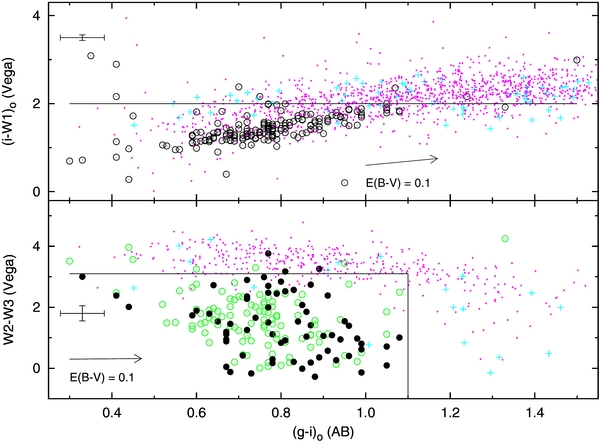
Figure 3. In the top diagram, the reddening corrected color formed by the SDSS i band and the WISE W1 band (both on the Vega system) are plotted against (g − i)o color for the same samples of 178 GCs (open circles) and 1325 galaxies (plusses and dots) as Figure 2. The objects that lie below the line in the top diagram are plotted in the bottom diagram, which is a plot of the color formed by the WISE W2 and W3 bands. The solid and open circles depict measurements and upper limits on W2 − W3, respectively. The objects that lie within the rectangle in the bottom diagram are considered GC candidates. They include ∼90% of the GCs and ∼9% of the galaxies that are plotted in the top diagram. To preserve clarity, only average error bars are plotted.
Download figure:
Standard image High-resolution imageGalaxies that are still forming stars can also resemble M31 GCs in visual appearance, and their V − K or i − W1 colors may not be particularly red because of the contributions from young stellar populations. Star-forming galaxies with rich populations of young stars may be distinguished from GCs by their UV fluxes. Bianchi et al. (2007) showed in their Figure 5 that the color NUV − g, where NUV is the near UV band (λeff = 2271 Å) measured by the GALEX satellite and g is the SDSS g band, separates blue galaxies from theoretical calculations of old SSPs of the same g − i color. We show in Figure 2 that the same plot separates many galaxies from M31 GCs. At the same g − i color, red galaxies and GCs may have similar NUV − g colors. In many cases, these red galaxies can be separated from GCs by their i − W1 colors.
The hot and luminous stars of a star forming galaxy not only cause a large UV flux and a blue NUV − g color, but they also warm the dust and excite emission from the polycyclic aromatic hydrocarbon molecules in the interstellar medium. Consequently, the SEDs of star forming galaxies have a prominent upturn in IR flux, which is not seen in the SEDs of E galaxies (Assef et al. 2010) and presumably GCs. Star-forming galaxies separate from E galaxies in the W2 − W3 color, where W2 and W3 are, respectively, the 4.6 and 12 μm bands measured by WISE (Yan et al. 2013). We show in Figures 2 and 3 that this color is also useful for separating galaxies from M31 GCs. This is true even if the W3 measurement is only an upper limit, and consequently the color index W2 − W3 is an upper limit. Since GCs have bluer W2 − W3 colors than star forming galaxies, an object whose upper limit on W2 − W3 is below the dividing line between GCs and galaxies is possibly a GC. However, a real GC, particularly a faint one, may have an upper limit on W2 − W3 that is above the cutoff, and this leads to some attrition of real clusters (see Figures 2 and 3). Since non-star-forming galaxies may also have blue W2 − W3 colors, it is necessary to use another criterion, e.g., i − W1 color, in combination with W2 − W3 to obtain a nearly pure sample of GCs.
When accessing the GALEX catalogs, we adopted a matching radius of 6 0, and if more than one NUV observation was listed, we calculated a weighted average using one over the square of the listed errors as the weights. The WISE photometry for the objects under study was obtained by comparing their positions with sources in the WISE ALL SKY catalog. Positions that agreed to within 50 were considered a match. At the resolution of the WISE observations (61, 64, and 65 in the W1, W2, and W3 bands, respectively; Wright et al. 2010), the great majority of the M31 GCs are unresolved. This appears to be also true of the majority of the galaxies that that fall within the magnitude and color ranges that we have adopted. Consequently, we have adopted the magnitudes in the WISE ALL SKY catalog that were obtained by point-spread function fitting rather than attempting to match particular objects to the measurements provided for several different aperture sizes.
To demonstrate the validity of our techniques, we compiled the following samples of GCs and galaxies. From the Kang et al. (2012) catalog of old M31 GCs with GALEX NUV magnitudes, we selected the 158 that have Rgc ⩾ 3 kpc. By excluding clusters that have smaller values of Rgc, we avoided ones that lie in fields with large amounts of background light and/or large reddenings and reduced the likelihood of confusions with other objects that have appreciable UV or IR fluxes. To see if there is a zero-point offset in NUV mag between the measurements by Kang et al. (2012) and the GALEX catalogs, we selected 33 M31 GCs that appear to be well separated from other sources. For these GCs, the mean difference in the sense catalog—Kang et al. is −0.06 ± 0.03. Because this difference is of low statistical significance and is small compared to the difference in NUV − g between GCs and most galaxies, we have ignored it. We supplemented the sample drawn from Kang et al. (2012) with 20 additional clusters from the catalog of Huxor et al. (2008), which were also in the GALEX catalogs. One sample of galaxies was selected from the RBCv5 (Galleti et al. 2004, 2012 edition). Because these objects are listed in the RBCv5, at least one previous study of the M31 GC population considered them to be likely GCs, but now they are unquestionably identified as galaxies. They are a sample of galaxies whose appearances resemble GCs, and 66 of them met our color and magnitude criteria for GC candidates. Since this is relatively small number, we selected 1259 objects from a ∼10 deg2 region of our survey that we believe are probably galaxies on the basis of visual inspection of the SDSS images alone, since we have neither redshift measurements nor very high resolution imaging for them. We excluded from this sample the bright and/or very obvious galaxies in order to obtain a sample of objects that might be confused with M31 GCs if they were more distant or viewed with worse resolution than the SDSS.
Since not all candidate GCs have GALEX measurements, the GC selections that can be made with both GALEX and WISE observations are shown in Figure 2 and with WISE observations alone in Figure 3. The top panel of Figure 2 is modeled after Figure 5 in Bianchi et al. (2007), and it shows that the sample of old M31 GCs form a sequence that is separated from most galaxies. Comparison with Figure 5 in Bianchi et al. (2007) suggests that the galaxies with (g − i)0 ≲ 1.1 are primarily star-forming ones, and consequently, have bluer (NUV − g)0 colors than the GCs, which resemble old, metal-poor SSPs. At (g − i)0 > 1.1, the galaxy samples include some objects with red (NUV − g)0 colors that overlap with a few GCs. These red galaxies are probably Es (Bianchi et al. 2007). The curve in Figure 2 represents our dividing line between galaxies and GC candidates, and 96.1% of the GCs and 1.7% of the galaxies fall below this curve and therefore pass this test. In the middle diagram of Figure 2, we have plotted these objects that passed the test in the upper diagram. The horizontal line separates GC candidates from possible galaxies. Since the top diagram has already excluded most of the contamination from red galaxies, this diagram is somewhat redundant, but it does exclude a few red galaxies that passed the test based on (NUV − g)0. After this cut, 93.8% and 1.4% of the GCs and the galaxies remain. The use of the W2 − W3 color to exclude star forming galaxies is shown in the bottom diagram. The objects that are plotted in this diagram passed the cuts that are illustrated in the upper two. The horizontal and vertical lines outline the region occupied by most GCs (see also Figure 3), and after using this region to make the final cuts, 87.6% of the original number of GCs remain, but only 0.2% of the galaxies. Only 1 of the 3 galaxies that passed all three cuts were among the 66 selected from the RBCv5. Most of the GCs that failed one or more of the cuts are among the faintest and/or the most heavily reddened ones in the sample.
We have also investigated the separation of galaxies from GCs using only optical and WISE bands because ∼25% of our visually selected GC candidates do not have GALEX measurements. In the top diagram of Figure 3, we have plotted the same samples of GCs and galaxies as in the top diagram of Figure 2, and the horizontal line is the same dividing line that was plotted the middle diagram of Figure 2. Below this line are 95.5% of the GCs and 32.0% of the galaxies, and these objects are plotted in the lower diagram of Figure 3. The horizontal and vertical lines in the lower plot, which are the same as the ones in Figure 2, provide the final cuts on the samples. They enclose 89.9% and 8.8% of the original samples of GCs and galaxies. A comparison with the above results shows, not surprisingly, that it is better to have in addition the cut by (NUV − g)0 color. Nonetheless, the cuts by (i − W1)0 and W2 − W3 are useful for removing the majority of galaxies from a sample of candidate GCs. The positions of the lines that are used to make the sample cuts are somewhat arbitrary, and one could set them so that a larger fraction of the galaxies are excluded at the expense, however, of removing more GCs.
3.3.2. Photometric Redshifts
The spectroscopic measurement of redshift (z) has been one of the best techniques for separating M31 GCs (e.g., Caldwell et al. 2009) from galaxies, because most galaxies of similar brightnesses have much larger z's. Photometric z's can be estimated from the broad-band colors of galaxies, and while they are much less precise than spectroscopic ones, they provide another tool for removing galaxies from a sample of GC candidates.
Data Release 10 of the SDSS (Ahn et al. 2014) provides two estimates of z that are based on the five SDSS color bands for objects in the Galaxy catalog, "Photoz" and "PhotozRF" and their errors.3 Because Photoz is on average about 0.015 lower than PhotozRF for the M31 GCs, we use only Photoz here. The Photoz values were determined by comparing the magnitudes of the objects in the five SDSS bands to the colors of galaxies in a training set of more than 850,000 galaxies with spectroscopically determined z. There are probably few if any GCs in this training set, and consequently one cannot expect the technique to produce reliable z values for GCs. What matters for our discussion of GC-galaxy separation is that the technique assigns consistently low values of z, albeit much larger than their real values, to the M31 GCs, and higher values to many galaxies of comparable brightness and color.
The diagrams in Figure 4 show plots of Photoz against reddening corrected r band magnitude (r0) and against (g − i)0 color. Except for the few galaxies not plotted because they have Photoz >3, the sample of galaxies is the same as the one used in Figures 2 and 3. Most of the GCs that are plotted in Figure 4 are the ones in Figures 2 and 3 that lie within the SDSS footprint. Seven additional clusters from Huxor et al. (2008) that have Rgc > 3 kpc and lie within the footprint have been added. These clusters were not plotted in the Figures 2 and 3 because they lack GALEX observations.
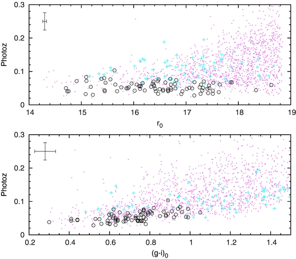
Figure 4. For 84 GCs (open circles), 66 galaxies from the RBCv5 (plusses), and ∼1200 other galaxies (dots), Photoz is plotted against r0 (top diagram) and against (g − i)0 (bottom diagram). Note that in both diagrams the GCs lie at the lower boundary of the distribution of galaxies. The error bars depict the average values of the random errors.
Download figure:
Standard image High-resolution imageThe top diagram in Figure 4 shows that except for two GCs that have r0 < 16.0 (B006 and B407, Photoz = 0.083 and 0.103, respectively), the GCs have Photoz <0.08. At r0 < 16.0, there is little separation between GCs and galaxies, but this is not of much concern because the images of most of these relatively bright galaxies have obvious disks or other features that clearly distinguish them from GCs. Moreover, the GCs in this magnitude range are very luminous (Mr < −8.4) and large, if they are at the distance of M31. In general, these GCs are the ones most easily resolved into stars in the SDSS images. As r0 increases, the range of the Photoz values of the GCs remains unchanged, while many more galaxies have large Photoz, as expected for a sample of galaxies. Photoz becomes a useful separator of galaxies and GCs in the magnitude range (r0 ≳ 16) where it is difficult to separate them in the SDSS images. The bottom diagram in Figure 4 shows that the range of Photoz for the galaxies increases substantially with (g − i)0. Among the GCs, Photoz increases only slightly with (g − i)0, and at every (g − i)0, the GCs lie at the lower boundary of the galaxy distribution.
If an object has a higher Photoz than the GC sequences in the diagrams in Figure 4, then it is most likely a galaxy and not a M31 GC or a IGC in the Local Group. For example, in Figure 4 the plusses depict galaxies that are in the RBCv5, which means that at one time they were identified as GC candidates. The Photoz values of many of these objects are significantly larger than the confirmed GCs, which excludes them as likely GCs. If an object lies on the GC sequences in the diagrams, there is still some possibility that it is a galaxy and not a GC. The Photoz technique most is useful when it is used in concert with the methods that employed the GALEX and WISE measurements. In the example that employed only (i − W1)0 and W2 − W3 (see Figure 3), 8.8% of the original sample of galaxies remained in the sample after the cuts. If the objects with Photoz >0.08 are excluded, the percentage of galaxies remaining drops to 2.9%.
4. RESULTS AND DISCUSSION
As noted above, the visual inspection technique yielded 320 objects that we considered potentially GCs. After making the cuts by (NUV − g)0, (i − W1)0, and W2 − W3 that are illustrated in Figures 2 and 3 and after excluding objects that have Photoz >0.08, only seven objects remained. The positions and colors of these seven objects are listed in Table 1, none of which is included in the RBCv5. We are confident that six of these objects are GCs. While the seventh object (F), which is the faintest of the group, passed all of the above color tests, its photometry has relatively large errors and its visual appearance is not beyond doubt that of a GC. Consequently, we consider it a GC candidate.
Table 1. Positions and Colors of the Globular Clusters
| Name | R.A. | Decl. | ξ | η | r0 | (u − g)0 | (g − r)0 | (g − i)0 | (NUV − g)0 | (i − W1)0 | W2 − W3b | Photozc |
|---|---|---|---|---|---|---|---|---|---|---|---|---|
| (deg) | (deg) | (deg) | (deg) | (mag) | (mag) | (mag) | (mag) | (mag) | (mag) | (mag) | ||
| A | 5.14119 | 36.65953 | −4.4 | −4.5 | 17.44 ± 0.01 | 1.44 ± 0.09 | 0.52 ± 0.01 | 0.82 ± 0.01 | 3.00 ± 0.12 | 1.40 ± 0.04 | 2.58 | 0.068 ± 0.026 |
| B | 6.71750 | 38.74947 | −3.1 | −2.5 | 15.99 ± 0.00 | 1.49 ± 0.02 | 0.69 ± 0.01 | 1.01 ± 0.01 | 4.08 ± 0.36 | 1.65 ± 0.03 | 1.18 | 0.059 ± 0.033 |
| C | 7.86467 | 39.53942 | −2.2 | −1.7 | 17.33 ± 0.01 | 1.14 ± 0.02 | 0.45 ± 0.01 | 0.68 ± 0.01 | 2.93 ± 0.08 | 1.15 ± 0.05 | 2.61 | 0.036 ± 0.020 |
| D | 9.03580 | 39.29165 | −1.3 | −2.0 | 17.24 ± 0.01 | 1.22 ± 0.03 | 0.50 ± 0.01 | 0.73 ± 0.01 | 2.80 ± 0.20 | 1.23 ± 0.04 | 2.83 | 0.046 ± 0.026 |
| E | 9.61483 | 40.65835 | −0.8 | −0.6 | 18.26 ± 0.01 | 1.50 ± 0.13 | 0.67 ± 0.02 | 1.01 ± 0.02 | 3.91 ± 0.11 | 1.96 ± 0.05 | 2.70 | 0.058 ± 0.027 |
| Fa | 11.26744 | 31.63141 | 0.5 | −9.6 | 18.30 ± 0.02 | 1.52 ± 0.21 | 0.28 ± 0.03 | 0.49 ± 0.04 | 1.91 ± 0.19 | 1.09 ± 0.11 | 3.10 | 0.044 ± 0.018 |
| G | 22.20478 | 47.07277 | 7.8 | 6.3 | 16.98 ± 0.01 | 1.32 ± 0.04 | 0.54 ± 0.01 | 0.81 ± 0.01 | ... | 1.39 ± 0.04 | 2.27 | 0.057 ± 0.027 |
Notes. (i − W1)0 and W2 − W3 are on the Vega system. All other magnitudes are on the AB system. aGlobular cluster candidate bUpper limits cPhotoz is used as a color index, not as a measure of redshift.
Download table as: ASCIITypeset image
Further evidence that these objects are GCs is provided by the two color diagram that is formed by a plot of (u − g)0 against (g − i)0 (Figure 5). Old GCs lie on a well-defined sequence in this diagram, which we have illustrated by plotting in Figure 5 the same confirmed GCs that we plotted in Figures 2–4. We restricted the clusters to the ones that have E(B − V) ⩽ 0.10 in order to show that the GC sequence is intrinsically tight. According to the extinction values listed by SDSS for the objects in Table 1, which come from the analysis of dust maps by Schlegel et al. (1998), only G, with E(B − V) = 0.13, has E(B − V) > 0.10. To show that only a small minority of galaxies lie near the GC sequence, we have plotted in Figure 5 the same samples of galaxies that we plotted in Figures 2–4, most of which also have E(B − V) ⩽ 0.10. Figure 5 is of course analogous to the plot of (NUV − g)0 against (g − i)0 (see Figure 2), but it does not separate GCs and galaxies as well. It is nonetheless a useful consistency check. All six of the objects in Table 1 that we believe are GCs lie on the GC sequence in Figure 5. The GC candidate (F) lies off the sequence, but in a region which contains relatively few galaxies. If the colors of this object had small errorbars, it would be an unlikely GC candidate. However, the errors in its photometry are sufficiently large that one cannot rule out the possibility they alone have produced the offset from the GC sequence. This object passes the GC criteria that are based on (NUV − g)0, (i − W1)0, W2 − W3, and Photoz, and in visual appearance it resembles a low surface-brightness GC (see Figure 6), which is consistent with its relatively large half-light radius (Rh) and faint absolute r magnitude (Mr), if it is at the distance of M31 (see Table 2). The SDSS images of F resemble those of some of the M33 GCs that lie in its outer halo (e.g., the ones studied by Cockcroft et al. 2011). In angular distance, F is slightly closer to M31 (9 7) than to M33 (105).

Figure 5. In a two-color diagram formed by the SDSS colors, the seven objects in Table 1 (solid circles with error bars) are compared with confirmed GCs (open circles) and galaxies (dots and plusses; see caption to Figure 2). Six of the objects lie within the GC sequence. F, which we consider a GC candidate, lies off the sequence, but in an area where the density of galaxies is low. The (g − i)0 colors of B and E have been adjusted by 0.01 mag to separate them.
Download figure:
Standard image High-resolution image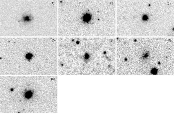
Figure 6. SDSS r-band images of the objects in Table 1. North is at the top, and east is to the left. The images are approximately 30'' by 45''.
Download figure:
Standard image High-resolution imageA mosaic of r-band images of the seven objects in Table 1 is shown in Figure 6. To construct this figure, we downloaded their "corrected" fits images from the SDSS Web site, which are sky-subtracted. These images show that the objects span ranges in magnitude, size, and amount of resolution into stars. The values of Mr and Rh (see Table 2) quantify the first two properties. Also listed in Table 2 is the projected distance from the center of M31 (Rgc), and all of the parameters in Table 2 were calculated assuming a distance of 780 kpc (McConnachie et al. 2005). To estimate Rh, we followed the same procedures as Paper I and used the r-band light profiles provided by SDSS. Cubic splines were fit through the cumulative distribution of the flux with radius, and the radius that enclosed 0.5 of the total was adopted as Rh. For GCs that are similar to the ones measured here, this procedure produces values of Rh that agree to within 15% with ones determined from images from the HST (see Paper I). In the classification scheme of Huxor et al. (2008), the values of Mr and Rh of the new clusters are typical of the "classical" GCs as opposed to "extended" GCs, which at the same absolute magnitudes have larger Rh (typically >15 pc; Tanvir et al. 2012).
Table 2. Properties of the Globular Clusters
| Name | Rgc | Mr | Rh |
|---|---|---|---|
| (kpc) | (mag) | (pc) | |
| A | 86 | −7.0 | 8.5 |
| B | 54 | −8.5 | 4.2 |
| C | 38 | −7.1 | 4.1 |
| D | 32 | −7.2 | 4.1 |
| E | 14 | −6.2 | 5.6 |
| Fa | 131 | −6.2 | 10.1 |
| G | 137 | −7.5 | 6.1 |
Note. aGlobular cluster candidate.
Download table as: ASCIITypeset image
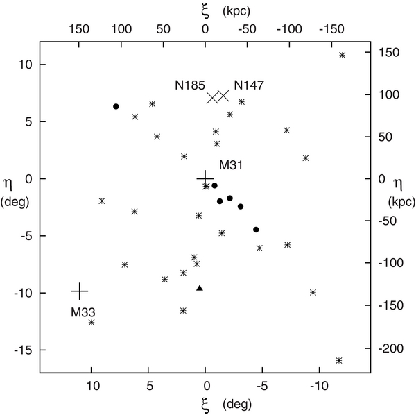
The quantities ξ and η in Table 1 are the angular distances from the center of M31 in the directions of R.A. and decl., respectively. They are plotted in Figure 7, where the M31, M33, and the M31 satellite galaxies are also plotted. Three of the new GCs, and possibly four if F is a GC, have Rgc ⩾ 50 kpc. They increase the already much larger population of distant GCs that have been discovered in M31 than in the MW. Since these GCs are more luminous than five of the six MW GCs that have galactocentric distances >50 kpc, they also increase the disparity between M31 and the MW in the properties of their distant GCs (e.g., Huxor et al. 2011). One can see from Figure 7 that while these new GCs lie far from the center of M31, they are within the same area of the sky as several satellite galaxies, which have distances and radial velocities that are consistent with being gravitationally bound to M31.
Figure 7. Positions in the sky of the new GCs (solid circles) and the GC candidate (solid triangle) with respect to the center of M31 (cross). The projected distances in kiloparsecs were calculated assuming 780 kpc for the distance to M31. The locations of M33 (plus), N147 and N185 (crosses), and the dSph satellite galaxies (asterisks) are indicated. The approximately linear distribution of the GCs is a consequence of the geometry of our search region.
Download figure:
Standard image High-resolution image
One of our objectives for this project was to find IGCs. On the basis of sky position alone, none of the GCs that we have found is likely to be a IGC, although this cannot be entirely ruled out until their distances and radial velocities are measured. IGCs may exist in the very remote regions of M31 where we have not searched, or they may be so faint in magnitude and/or surface brightness that they escaped our detection.
We gratefully acknowledge the technical support provided by Gabriele Zinn throughout this project, which greatly facilitated its completion. This research has been supported by NSF grant AST-1108948 to Yale University. This project would not have been possible without the public release of the data from the Sloan Digital Sky Survey III and the very useful tools that the SDSS has provided for accessing and examining the publically released data. Funding for SDSS-III has been provided by the Alfred P. Sloan Foundation, the Participating Institutions, the National Science Foundation, and the U.S. Department of Energy Office of Science. The SDSS-III Web site is http://www.sdss3.org/.
SDSS-III is managed by the Astrophysical Research Consortium for the Participating Institutions of the SDSS-III Collaboration including the University of Arizona, the Brazilian Participation Group, Brookhaven National Laboratory, University of Cambridge, Carnegie Mellon University, University of Florida, the French Participation Group, the German Participation Group, Harvard University, the Instituto de Astrofisica de Canarias, the Michigan State/Notre Dame/JINA Participation Group, Johns Hopkins University, Lawrence Berkeley National Laboratory, Max Planck Institute for Astrophysics, Max Planck Institute for Extraterrestrial Physics, New Mexico State University, New York University, Ohio State University, Pennsylvania State University, University of Portsmouth, Princeton University, the Spanish Participation Group, University of Tokyo, University of Utah, Vanderbilt University, University of Virginia, University of Washington, and Yale University.
This publication makes use of data products from the Wide-field Infrared Survey Explorer, which is a joint project of the University of California, Los Angeles, and the Jet Propulsion Laboratory/California Institute of Technology, funded by the National Aeronautics and Space Administration.
Footnotes
- 1
- 2
We thank the referee for bringing this paper to our attention.
- 3