


ABSTRACT
We present a new analysis of 843 photographic plates of Pluto taken by Carl Lampland at Lowell Observatory from 1930–1951. This large collection of plates contains useful astrometric information that improves our knowledge of Plutoʼs orbit. This improvement provides critical support to the impending flyby of Pluto by New Horizons. New Horizons can do inbound navigation of the system to improve its targeting. This navigation is capable of nearly eliminating the sky-plane errors but can do little to constrain the time of closest approach. Thus the focus on this work was to better determine Plutoʼs heliocentric distance and to determine the uncertainty on that distance with a particular eye to eliminating systematic errors that might have been previously unrecognized. This work adds 596 new astrometric measurements based on the USNO CCD Astrograph Catalog 4. With the addition of these data the uncertainty of the estimated heliocentric position of Pluto in Developmental Ephemerides 432 (DE432) is at the level of 1000 km. This new analysis gives us more confidence that these estimations are accurate and are sufficient to support a successful flyby of Pluto by New Horizons.
Export citation and abstract BibTeX RIS
1. INTRODUCTION
With the discovery of Pluto over 80 years in the past, it is easy to imagine that its orbit should be a well known quantity by now. When reminded, most people would recognize that we have been measuring Plutoʼs position for only about 1/3 of its orbital period. It is then somewhat amazing that we have a spacecraft on its way for a flyby. Upon further reflection, it is useful to point out that due to its eccentric orbit, Pluto has actually traversed more than half of its orbit when measured in ecliptic longitude. Indeed, opposition has moved from January to July since Plutoʼs discovery due to the occurrence of perihelion in that range of time. From here, opposition will take another 160 years to complete the cycle as Pluto finishes its first full orbit since discovery.
We certainly do not have any difficulty predicting Plutoʼs position in the sky for the purposes of telescopic study. Even back in the early 1980s the position was known to be good to a few arcseconds, easily good enough for identification and acquisition. Since that time the ephemeris has steadily improved. The one area where the position of Pluto remains a challenge is in predicting stellar occultations. Current predictions are good enough to get observers somewhere in the shadow but high-precision targeting, such as making multiple chord measurements of the 100 km (4 mas) central flash region, are not routinely possible. There is certainly a complication introduced by the fact that we are really dealing with a double planet and at the level of precision desired significant challenges remain.
From the concern over stellar occultation predictions it is a small step to be concerned over the actual state of the knowledge of the orbit in the context of the upcoming New Horizons flyby. At the heart of the mission design and its encounter plan is the need to know the time of closest approach. Furthermore, for building a robust encounter plan we also need to know the uncertainty on that time as well. To put this in perspective, the encounter at 2015 July 14 11:50:00 UTC (spacecraft time) happens with a flyby distance of 13,695 km from the center of Pluto and a flyby speed of 13.78 km s−1 (Guo & Farquhar 2008; Young & Stern 2009). Getting the flyby right all comes down to the heliocentric distance of Pluto at the time of encounter. We know the position of New Horizons very accurately due to radio tracking data. We only know Plutoʼs distance from the knowledge of its orbit. The current adopted 1-σ uncertainty in Plutoʼs distance is 1378 km (corresponds to a time-of-flight error of 100 s, from the New Horizons Mission System Requirements Document). If it can be shown that the actual uncertainty is consistent with this adopted number, the encounter plan is expected to achieve all mission goals (and more). If the error is significantly larger, that error will lead to very large angular errors (relative to the trajectory) for the location of the objects in the Pluto system and large portions of the best near-encounter observations are at risk for missing their targets.
Anyone that observes Pluto these days knows the challenges due to its current low galactic latitude. In addition, the galactic longitude puts it near some of the most crowded parts of the sky. The background star density has been on the rise since 2000 and will soon begin to slowly taper off. While difficult for most observations, the increase in stellar background has led to a significant increase in the number of stellar occultations. While we are certainly more confident in our predictions than we were for the occultation seen back in 1988, these more recent events have still proven difficult to predict. To put this in perspective, Pluto occultation events seem to be good only to about 1000 km or so, slightly less than a planetary radius. Predictions of Triton occultations, on the other hand, can be as good as 100 km. This comparison is notable since Pluto and Triton are at similar heliocentric distances. The reason for the difference is hard to identify but consider that we have astrometry for Neptune (and thus the system barycenter) for longer than one full orbit period. Prediction efforts by Assafin et al. (2010) provided a summary of the astrometric constraint provided by all of the stellar occultations between 2005–2009. After all, given an occultation, you know the relative position of the star and Pluto to a few km. If you think you know the positions of the stars then you have information that can be compared to current orbits. Their results showed a clear trend in declination relative to DE418. There are many possible explanations for this error but the most worrisome is that perhaps the current orbits have some error in the current distance to Pluto.
With a project of the importance of New Horizons, it is well worth the effort to make sure we have the best possible orbit as well as understanding just how accurate the Pluto ephemeris is. The focus of this work is to rule out a large, unrecognized systematic error in the orbit fitting to date. This type of error can come from any number of places but the one thing we can bring to the problem that will help is new astrometric data. The Gaia mission (c.f. Prusti 2012) would definitely resolve all our questions about Plutoʼs orbit. While Gaia will directly measure Pluto, its primary importance is in the high-precision star catalog. Having that catalog will allow a re-reduction of all existing data and return a much better orbit estimate. Unfortunately, those results will not be available until well after encounter. Even at the time of New Horizons launch in 2006, it was not obvious that Gaia would be able to help. Near that time, Buie was discussing the concern over the orbit with Brian Skiff (both at Lowell Observatory at the time). Skiff pointed out the existence of a large collection of photographic plates containing Pluto images that were taken by Carl Lampland, also of Lowell Observatory. This plate collection began shortly after the discovery of Pluto and continued up to within a few weeks of Lamplandʼs death in 1951. This plate collection and the availability of significantly better astrometric support catalogs provided the new data set desired to address the question of Plutoʼs orbit. It was hoped that by bringing in a new dataset to the earliest epochs of our data on Pluto that we might be able to find or eliminate a large systematic error.
This paper provides the details of the plate collection, analysis, and collection of astrometry. We then go on to compare to existing orbit fits and then finally to a new orbit fit including the new data. This work also serves to document the plate collection and all of its associated information that is archived in the Lowell Observatory collections.
2. PLATE PROCESSING
All of the Lampland plates were taken with the Lowell Observatory 40 inch reflector. This facility was located on the main observatory grounds in Flagstaff. The telescope was an f/6 reflector with a Newtonian optical design. According to observatory lore, sometime after Lamplandʼs death there was an attempt made to cut a hole in the primary mirror to convert it to a Cassegrain-like configuration. Unfortunately, there was apparently a lot of internal stress in the glass of the mirror and during the cutting process the mirror was completely destroyed thus ending the life of that facility. The telescope framework remained in its dome until the 1990s at which time it was relocated to an outdoor display on the observatory grounds.
The telescope itself was not particularly well-suited to astrometric work in that its field of view (FOV) was significantly smaller than common for its time. The plates are 4 × 5 inches (10 × 13 cm) with a plate scale of 39.5 arcsec mm−1. Thus the full FOV was 1°.1 × 1°.4, still large in comparison to todayʼs CCD cameras but small compared to instruments then. The primary difficulty with this FOV is in finding sufficient astrometric reference stars from which to derive a plate solution. The complete time history of this plate collection is summarized in Figure 1. In this figure, each plate is marked with a dot superimposed on the motion of Pluto to show the density of coverage. This graph shows the variable coverage within and between years. In the first decade after discovery the astrometric monitoring was more complete. Some effort was made both by Lampland and then later by H. Giclas to extract astrometry from these plates. Indeed, the current astrometric record does include some measurements from these plates already. Without the pressing need of New Horizons, these data would probably still be sitting in the plate vault at Lowell Observatory as an unrecognized resource.

Figure 1. Graphical summary of the Lampland Pluto plates. The curved lines shows the path of Pluto on the sky over the range of the plate collection. The blue portions of the curve show when Pluto has a solar elongation greater than 60° and yellow when too close to the Sun and unobservable. The magenta triangles mark the time of opposition each year with a label below showing the year of opposition connected by a faint gray dashed line. The observations begin at the time of discovery and end with Lamplandʼs death.
Download figure:
Standard image High-resolution imageThis effort of reprocessing the Lampland plates was also precipitated by the release of the UCAC2 astrometric catalog (Zacharias et al. 2004). The improvement provided by this and subsequent catalogs was to have proper motions good enough to permit accurate reductions of these old plates. Thus, even though the catalog epoch is far from the time of the Lampland plates, the proper motions gave hope that a new reduction of those plates against UCAC2 would yield significantly better astrometry than what was possible at the time the plates were taken. The Hipparcos (Perryman et al. 1997) and Tycho-2 (Høg et al. 2000) catalogs were not considered because of the field distortions expected in the images seemed to require a denser catalog.
The plates needed to be digitized before processing as well as collecting all the ancillary data related to these plates. There are three sources of information for each plate and we created a fourth during processing. First, the plates themselves have the date and plate number written on the emulsion. Second, there is information often written on the plate sleeves. At a minimum this information is merely just a copy of the information written on the plate. However, the plate sleeve also indicates how many plates are in the set for that night. Additionally, there are often notes written by either Lampland or Giclas that describe the quality of the image, provide information about their own plate analysis, or an explanation about some calibration effort recorded on the plate. For example, there are quite a few plates that are double exposures. The first exposure is on the Pluto field and its start time is recorded. Then, a second exposure was taken at a different location on the sky to superimpose a selected area (SA) field on the same plate. Actually, we do not know if the SA image is first or second but it does not matter for our efforts. For these fields, care had to be taken to make sure the appropriate set of stars was used for the plate solution. This provided considerable confusion for automated astrometry systems that were used in certain steps of the processing. The third source of information is a logbook, mostly in Lamplandʼs handwriting that provides additional information such as comments on the quality of the night and most importantly, the start time of the plate. According to observatory lore, Lamplandʼs methodology was to document each plate or each night of plates on a note card. Sometime later the information on these cards would be transcribed onto either the plate sleeves or logbook, or both. Perhaps in the earliest days, this step was done closer in time to when the plates were taken but in later years it seems to have been common to wait for the completion of the observing season before writing up the information. This is the explanation given for the lack of information in the logbook for data for the last 4 years: Lampland died before transcribing the last set of cards. These cards had to have been known to Giclas during his analyses since 72 plate sleeves in the last years have a start time written down in Giclas' handwriting. An exhaustive search of Giclas' collected notes failed to uncover these cards, though copious information was found for his work on the astrometric reductions. There remain 162 plates from 1948–1951 that have no start time noted and thus cannot be usefully processed to extract Pluto astrometry. These plates were digitized along with the rest just in case this information turns up someday. These plates are also still useful for photometric analysis since we can use Plutoʼs position to infer a start time. The last source of information was generated during our processing of the plates. At the start of this project, the plates were still housed in their original sleeves. These sleeves show obvious signs of yellowing and other deterioration. As the plates were processed we relocated the plates into archival quality sleeves and transferred the date and plate number information to the new sleeves. We also assigned each plate a unique integer number (mostly sequential in time) to each sleeve. This number serves a very useful purpose to bind together all the known plate information into a master database created for these plates.
In the first step of this project we used a high-end commercial flat-bed scanner to scan the plates, the plate jackets, and the logbooks. The hope was that by using a top-of-the-line scanner, the scanned images would be of sufficient quality to support the astrometric reductions. Sadly, this supposition turned out to be incorrect. Regardless, this step served many useful purposes. We now have digital copy of all the ancillary information and there is a good browsing set of images of the plates that required minimal processing. The scans of the plates, while ultimately useless for astrometry, are still quite valuable for extracting photometric information but that remains for a future project. The glass side of the plates were cleaned prior to scanning. All of the plates were found to be covered in what appears to be tobacco smoke residue (a yellowish-brown film). There must be a similar coating on the emulsion side but this cannot be removed by any methods currently available. There were also handwritten marks such as arrows or circles where either Lampland or Giclas marked the location of either Pluto or an astrometric reference star. These marks were also removed though a few plates still show some remnant marks, particularly near (but not on) Pluto.
The plate solutions for this first attempt seemed useful at first glance but a more detailed examination of the post-fit residuals showed systematic patterns in the axis parallel to the scan bar motion in the scanner. The residuals were quasi periodic with a peak-to-peak amplitude of about 1.5 arcsec and was not repeatable in amplitude, phase, or even shape from one plate to the next. Despite considerable effort we did not find a way to remove this signature. As a final check, the Pluto astrometry derived from these sub-optimal plate solutions was checked against JPLʼs DE418 ephemeris. There were large systematic shifts in these data that could not be taken out by a refit to the data, demonstrating conclusively that we needed better quality scans of the plates.
In time, we identified two groups concerned with making high-quality digital scans of photographic plates. The first group at the Royal Observatory of Belgium has the DAMIAN system with a small imaging array detector on a high-precision mechanical stage (Robert et al. 2011). The stage is stepped across the plate taking numerous small images. Through precise knowledge of the stage mechanism a final relationship is derived that relates a pixel position in a single small image to its absolute location on the plate. More details about DAMIAN can be found in Robert et al. (2011). We did test scans on a few plates. One of the tests was to scan the plate twice, with a 180° rotation between scans to see that the distances between stars were invariant between the scans. This system passed the test showing these scans would work very well. One down side of this system is that it took a relatively long time to scan. One estimate indicated it would take many months to work through the entire plate collection.
The second group is at Harvard. Jonathan Grindlay and his team developed the DASCH scanner (Grindlay et al. 2009; Los et al. 2011) for the purpose of digitizing the Harvard plate collection. Like DAMIAN, it has a camera mounted on a moving stage and builds up a scan of the plate by taking a series of sub-images in a raster pattern. This system was designed from the start to do two things differently from DAMIAN. First, the output of their data processing pipeline assembles the images into a large monolithic image that can be treated just like any other digital astronomical image. Second, it was designed to be very fast. This system is so fast that for these plates, the scanning rate was limited by the time it took to load and unload the plates between scans. The peak rate for this system was about 1 plate per minute. As with DAMIAN, the test scans showed the system would deliver astrometrically useful data. In the end we chose to scan the images with the DASCH scanner. The plates were scanned over the course of three days in 2013 September.
The digitized output products from the DASCH system include the original sub-rasters in raw form, all calibration images (bias, dark, flat fields), and the final assembled mosaics. All images are saved in FITS format and the unique plate number assigned to each plate makes up part of the file name. The images are scanned at a scale of 10.988 microns/pixel or roughly 0.4 arcsec/pixel. This pixel density over-samples the grains of the photographic emulsion. The image array size came out to be 8684 × 10,995 pixels or 0.96 by 1°.22 across. The ancillary data for each plate was added to the header during the scanning process. The mosaics were also run through an automatic astrometric reduction to determine a world coordinate system (WCS) mapping from pixel to sky coordinates. Had this been 100% effective the subsequent astrometric reduction would have been trivial. Unfortunately, there were a large enough fraction with bad solutions that the WCS solutions had to be re-done with the interactive astrometric reduction tools (astrom.pro) from Buieʼs IDL library.3 While this path required more manual effort, some of the plates (e.g., double exposures) could not be processed in any other practical way. This second-pass solution was also written to the header of each image.
It is worth making a few comments about the ancillary data for each plate. The most important item required to make any plate useful for astrometric data is the time when the exposure was taken. The timing information was obtained manually by Lampland, in the form of a start and end time noted from some handy timepiece. The exposures were always started at the beginning of a minute or at 30 s into the minute. Exposure durations were always some integer number of minutes. Most exposures were 10–15 minutes in duration but there were some as short as 5 minutes and some as long as 20 minutes. In the end, the quality of the astrometry of these plates are only as good as the timing. A typical rate of motion at opposition for Pluto is about 3 arcsec/hour. For instance, to get astrometry good to 0.1 arcsec requires that the timing is known to better than 2 minutes. Again citing Observatory lore, the survey that led to Plutoʼs discovery (Tombaugh 1946) brought a new level of rigor to the handling of time at the observatory. Prior to a nightʼs observing, someone (presumed to be Tombaugh) would walk down to the train station and synchronize a timepiece with the railroad clock and then bring it back up to the observatory grounds just a couple of kilometers away. This distributed time was used by anyone observing that night to minimize timing errors. It may be stretching the point to say the timing is good to a second but with this scenario it should not be significantly worse. Thus, we estimate the intrinsic noise added to the astrometry from timing errors to be near 1–2 mas.
There were also challenges in the interpretation of the logged times for the plates. The logbook indicates that all times are "Astronomical Time" without providing any explanation. The hour angle and airmass were provided so it is possible to work backward from Plutoʼs position to estimate when the plates were taken. AT was treated the same as if it were UTC except for a constant offset (UTC−AT) that was assumed to be an integral number of hours. This offset was determined to be +7 hours. There were changes in how the times were recorded over this time, though. Most notably was in handling how a time was recorded before and after midnight. Numerous cases were identified, prior to 1933 January 24 where the wrong date was inferred from the log for pre-dawn observations. These cases were easy to spot in the astrometric residuals against Plutoʼs ephemeris allowing a correction to be made to the date.
The final images that were readied for astrometric processing are named for the UT date of the night of observation, followed by the plate number during the night (e.g., 19300401.002). Note that the first pass processing had not yet discovered the date confusion in some of the nights and had used the date listed in the log book for each of plate identification. Most of the time this leads to a date that is one day earlier. This point is mentioned since both epochs of scans are saved in the archives at Lowell Observatory.
3. ASTROMETRIC REDUCTIONS
Processing the digitized images to extract Pluto astrometry uses methods that are quite similar to those used for CCD-based image data. As with CCDs, the pixelation defines a fundamental raw coordinate system intrinsic to the data. The following sections detail the processing steps and considerations leading up to the final Pluto astrometry.
3.1. Source Detection
The digitization process accurately records the density (or opacity) of the photographic plate. However, the correspondence between density and brightness is quite nonlinear and has a much lower point-by-point dynamic range than a digital detector. Besides being very oversampled, the images from astronomical sources have a very different character. The most important difference is that the size of the image formed from a source varies with the brightness. Sources right at the detection limit are very small (∼4 pixels) and the size increases from there based on brightness. Useful source images varied in size from 4 to 25 pixels, FWHM.
All images were scanned for point sources with the IDL routine findsrc.pro. This method is described in more detail in Buie et al. (2011) but basically scans the image for pixels in the image that exceed the nearby noise in the image by a specified threshold level. The background and noise level for each pixel is measured at four positions from a 1 × 10 pixel array window that is above, below, left, and right from the pixel and is separated at its closest point from the pixel being tested by 16 pixels. Any pixel that exceeded 8σ from the sky mean in at least three directions is flagged as a pixel of interest. This pixel interest image is eroded so that groups of adjacent pixels are reduced to a single pixel representing a single source at the position peak value of the group such that no two sources can be closer than 16 pixels. This eroded list is the resulting raw list of sources in the image. There can, of course, be false detections at this step but this problem was minimized by the choice of the control parameters.
3.2. Source Measurement
A special routine was developed for measuring these photographic plate images. Traditional CCD-based tools (basphote.pro) were poorly suited to images where object size is not consistent within the image. Instead, we used an algorithm derived from past experience with micro-densitometer measurements designed for photographic plates (photphot.pro). The method uses marginal distributions with a pair of one-dimensional Gaussian fits (x and y directions). The calculation yields a position, flux, and FWHM for each source along with uncertainties for all values. The uncertainties for the references stars were not used in this analysis, largely because the uncertainty in the astrometric fit was expected to be dominated by errors of the reference catalog. This method, used for decades on photographic plates, is ideal in that the FWHM of the image is not assumed or needed going into the calculation. The only variable of concern is the size of the region over which the marginal distribution is computed, in this case it was 16 pixels. The obvious utility of this method is that the flux is derived from the area under the fitted Gaussian curve that adapts to the size of the object. Admittedly, this measurement technique is easily tainted by nearby sources, such as when working in crowded fields. However, these data were not crowded and the vast majority of the sources are well isolated.
3.3. Initial Astrometric Fit
The plate center is assumed to coincide with the optical center for the fitting. The raw plate coordinates are then converted to normalized plate coordinates by subtracting the position of the center (4342, 5497.5) and then dividing by a normalization factor (14010.77 = diagonal length of digitized image). These normalized plates coordinates are used in the fit.
The positions of the astrometric calibration sources are from the USNO CCD Astrograph Catalog 4 (UCAC4) catalog (Zacharias et al. 2013). Much of the work in this step is associating a catalog source with a source in the image. For this, automatic pattern matching was used when possible but a significant number of plates required manual examination and field identification. The DASCH pipeline WCS solution was used as much as possible to minimize the work at this stage but roughly 40% of the plates required some sort of effort to get a good pattern match. One of the largest sources of difficulty was the degree of rotation between different plate scans. During the first scanning effort, the rotation was found to be extremely stable, presumably due to the fixed orientation of the plate holder on the telescope and the fiducial mounting arrangement in the first scanner. The DASCH system employs a clamp to hold the plates in place during scanning but the clamping process introduced a small random rotation to each plate as it engaged. This rotation was generally within 5° of some average value but this is the one weakness of the software Buie has developed for astrometry. That software was designed to take advantage of rotational stability that is normal for CCD imaging. When this is true, the software is extremely fast and reliable. When there are random rotations, the software has to work much harder to get a successful match, and at times requires manual intervention.
The catalog coordinates were then converted to tangent plane coordinates using an estimate of the coordinates of the plate center. A linear least squares fitting routine based on singular value decomposition (Press et al. 1992, p. 518) generated the fit for a given basis set. This routine (mysvdfit.pro) also does an iterative fit looking for unusual outliers from the fit, removes them, and refits the data. This iterative process continues until no further discrepant values remain. For most fits, there are 100 or more sources that contribute. No attempt was made to do any weighted fitting at this point. All sources are treated equally.
Of the basis sets attempted, a simple polynomial set worked sufficiently well and was adopted. Originally, it was hoped that this fit would be the final fit for each plate and would directly support the Pluto astrometry. For this reason, a fifth-order polynomial was chosen. The higher order terms were significant and necessary but somewhat poorly determined. Unlike the usual CCD process, there was no way to divine mean high-order terms due in large part to the intermediate step of scanning the plates where shifts and rotations were introduced into each plate scan. Still, the fits from this step served a very useful purpose in subsequent processing. The resulting fit was then written to the header of each image. This appears as a second, fully independent, WCS solution from that derived by the DASCH pipeline. An estimate of the photometric zero-point for each image is also saved to the header but this should not be treated as an accurate calibration value—it is meant merely as a guide.
3.4. Pluto Astrometry
It was common practice for Lampland and Giclas to work with just a fraction of a plate for their own piecemeal astrometric reduction. Those plates that were analyzed had black paper masks taped to them with squares cutout and centered roughly on the position of Pluto. The purpose of this method was to refrain from using the edges of the plates where the optical and spatial distortions grow ever larger. The wisdom of this approach is quite evident from the results of the fitting in the previous section. A fit over the entire plate is possible thanks to the increased density of the UCAC4 astrometric catalog and also due the computational ease made possible by todayʼs computers. However, just because a fit is possible does not make it the best choice for the Pluto astrometry.
A second step was employed that was patterned after the practices of Lampland and Giclas. In the analysis software, a region of interest (ROI) was defined for each plate based on the known ephemeris position for Pluto and then translated to pixel coordinates using the initial fit. This position was required to be more than 50 pixels from the edge of a plate for that plate to be processed. The ROI was then defined to be a square 4001 pixel region (26.7 arcmin) centered on Plutoʼs position. If this box extended over the edge of the plate it was truncated, resulting in a smaller box where Pluto was no longer in the center. Better results could, in principle, have been possible using just the Hipparcos or Tycho-2 catalogs but their density is insufficient to support this stage, thus requiring the use of UCAC4.
Using the initial fit, the pixel positions of the astrometric sources contained within the ROI were computed. The object aperture used for all sources was a 16 pixel radius circle. A local value of sky was computed for each source with an annulus having an inner radius of 26 pixels and an outer radius of 166 pixels (10–150 pixels beyond the object aperture). This sky value sets the baseline against which the marginal sums are computed for the sources and Pluto alike. The Pluto position was derived from first measuring local sky, then searching for the peak pixel position near the ephemeris position within a 11 × 11 box. With this position and sky value, the marginal sum was computed on the Pluto image.
At this point, the sample of sources was examined for bad measurements. Any source that returned a negative flux in either the x or y sum was discarded. Any source with a local value of sky that fell outside a normal distribution for all sky values was discarded. The x and y positions for the marginal sum was compared to the predicted location from the initial fit. Those differences that fell outside a normal distribution were discarded. Note that a simple shift between the two lists of positions would not eliminate any source as long as the shift is consistent among all sources. Next, the signal-to-noise ratio as measured by the x and y fluxes divided by the formal error of the x and y fluxes was required to be 20 or higher or they were discarded. Finally, the x and y positional error on all catalog sources were required to be smaller than 0.5 pixels. This second pass fit used the ephemeris position of Pluto as the tangent plane coordinate and a linear fit was applied to the surviving sources, again with an iterative fit that removed discrepant values. Due to the earlier filtering, this last-stage cleanup removed very few sources.
The regional linear fit was then used to convert the measured pixel location of Pluto to R.A. and decl. relative to the Earth mean equator (EME) and equinox of J2000.0 and then saved. Note that these measurements are really of the combined photo-center of the Pluto–Charon system. The step of converting these measurements to barycentric positions is left for later. The uncertainties recorded reflected the Pluto measurement errors only and do not include any uncertainties from the regional astrometric fit or from the catalog. Of the 843 plates scanned, 596 yielded astrometric measures on Pluto. Those that did not yield measurements either did not contain Pluto or were of insufficient quality to be worth measuring. Some of these were skipped due to insufficient information about the time the plate was taken. A few were simply ambiguous based on the logbook and plate cover notations. Most of this category date from the final three years of the collection where the exposure information could not be found.
The final results of the astrometric reduction are provided in Table 1. The displayed table is just an example for format but the entire dataset is available in the electronic supplement. The only thing omitted from this table stub is the file name of the archived image. All times for the data are presented as UTC by applying integer hour time corrections to the recorded times and give the mid-time of each exposure. The topocentric R.A. and decl. are shown along with their uncertainties. The observatory location was on the main Lowell Observatory campus. The position of the observatory was measured in the center on top of the dome to be N 35° 12 182, W 111° 39988, 2225 m on the WGS84 datum. The estimated uncertainty in this position is 4 m. For R.A., the uncertainty is in seconds of time and does not include a
  correction. For decl., the uncertainty is in arcseconds. These uncertainties estimate the errors in the measured position of Pluto and do not include any contribution from errors in the plate solution or the underlying catalog errors. The relative quality of the astrometric fit is given by
  and
and  , which is the unweighted
  for the fit in each tangent plane axis divided by the number of stars. These values are also equivalent to the rms of the post-fit residuals in arcseconds. The columns labeled
  and
and  give the formal uncertainty on the constant term of the ξ and η fits in arcseconds. The final column shows the number of good stars that were used in the local fit in the ROI around Pluto. It is important that some estimate for intrinsic errors of the plate solution be combined with these uncertainties or some other estimate of the catalog errors or these data will over constrain a solution. We discuss our approach for this final adjustment in Section 4.2.1.
Table 1. Pluto Astrometry
| UTC | R.A. | σα | Decl. |

|

|

|

|

|
Nstars |
| (sec) | ('') | ('') | ('') | ||||||
| 1930/02/27 03:34:00 | 07:20:33.933 | 0.005 | +21:56:56.75 | 0.06 | 0.087 | 0.068 | 0.053 | 0.053 | 358 |
| 1930/03/01 03:46:30 | 07:20:27.726 | 0.005 | +21:57:16.96 | 0.05 | 0.087 | 0.063 | 0.055 | 0.055 | 334 |
| 1930/03/02 04:56:30 | 07:20:24.632 | 0.004 | +21:57:26.98 | 0.05 | 0.081 | 0.064 | 0.050 | 0.050 | 407 |
| 1930/03/04 03:49:45 | 07:20:19.120 | 0.005 | +21:57:45.76 | 0.06 | 0.080 | 0.075 | 0.052 | 0.052 | 374 |
| 1930/03/04 04:18:30 | 07:20:19.083 | 0.007 | +21:57:45.84 | 0.11 | 0.077 | 0.071 | 0.074 | 0.074 | 182 |
| 1930/03/05 03:44:00 | 07:20:16.452 | 0.005 | +21:57:54.84 | 0.08 | 0.070 | 0.076 | 0.048 | 0.048 | 438 |
| 1930/03/05 04:07:00 | 07:20:16.415 | 0.005 | +21:57:54.97 | 0.07 | 0.078 | 0.079 | 0.054 | 0.054 | 343 |
| 1930/03/05 04:19:30 | 07:20:16.409 | 0.014 | +21:57:55.28 | 0.12 | 0.071 | 0.053 | 0.091 | 0.091 | 121 |
| 1930/03/05 04:32:00 | 07:20:16.359 | 0.005 | +21:57:55.40 | 0.09 | 0.081 | 0.074 | 0.067 | 0.067 | 225 |
| 1930/03/12 03:09:00 | 07:20:00.362 | 0.012 | +21:58:54.37 | 0.18 | 0.104 | 0.108 | 0.071 | 0.071 | 198 |
| 1930/03/12 03:19:00 | 07:20:00.349 | 0.012 | +21:58:54.32 | 0.11 | 0.103 | 0.099 | 0.069 | 0.069 | 208 |
| 1930/03/12 03:28:15 | 07:20:00.356 | 0.011 | +21:58:54.39 | 0.10 | 0.100 | 0.093 | 0.070 | 0.070 | 204 |
| 1930/03/13 02:45:00 | 07:19:58.502 | 0.008 | +21:59:01.59 | 0.20 | 0.099 | 0.088 | 0.080 | 0.080 | 155 |
| 1930/03/13 02:53:00 | 07:19:58.454 | 0.006 | +21:59:01.59 | 0.08 | 0.097 | 0.110 | 0.071 | 0.071 | 201 |
| 1930/03/13 03:01:30 | 07:19:58.430 | 0.016 | +21:59:01.77 | 0.13 | 0.114 | 0.088 | 0.085 | 0.085 | 139 |
| 1930/03/14 03:05:00 | 07:19:56.619 | 0.008 | +21:59:09.38 | 0.09 | 0.088 | 0.076 | 0.075 | 0.075 | 183 |
| 1930/03/14 03:14:00 | 07:19:56.605 | 0.009 | +21:59:09.08 | 0.15 | 0.107 | 0.094 | 0.072 | 0.072 | 196 |
| 1930/03/14 03:25:00 | 07:19:56.617 | 0.010 | +21:59:09.42 | 0.15 | 0.092 | 0.090 | 0.073 | 0.073 | 191 |
| 1930/03/15 02:44:15 | 07:19:54.913 | 0.006 | +21:59:16.53 | 0.06 | 0.090 | 0.088 | 0.063 | 0.063 | 255 |
| 1930/03/15 02:54:00 | 07:19:54.904 | 0.007 | +21:59:16.51 | 0.16 | 0.091 | 0.109 | 0.075 | 0.075 | 179 |
Note. All positions topocentric with the equinox of J2000 as defined by UCAC4.
Only a portion of this table is shown here to demonstrate its form and content. Machine-readable and Virtual Observatory (VO) versions of the full table are available.
Download table as: Machine-readable (MRT)Virtual Observatory (VOT)Typeset image
4. ORBIT
4.1. Comparison to Existing Orbits
Prior to fitting, the astrometry was checked against existing ephemerides. The scatter of the data against DE430 was 0.140 arcsec in R.A. and 0.165 arcsec in decl. Figure 2 shows the offsets as a function of time for the entire data set. The gaps in the data occur when Pluto is in conjunction with the Sun. There is at least one data point every year between 1930 and 1951. Table 2 provides a numerical summary of the offsets by year. Each line in the table is for one apparition of Pluto with the approximate time of opposition to the nearest 0.1 of a day. In the table are shown the number of observations (N), the mean offset between the observations and ephemeris ( and
and  ), the scatter (average of the absolute value of the differences,
  and
and  ), and the standard deviation (σ) of the differences. The left side of the table shows the statistics for DE430. The comparison to DE432 will become clearer in Section 4.2.
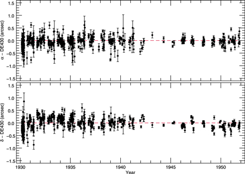
Figure 2. Comparison to DE430. The astrometry from the Lampland plates relative to DE430 is plotted as a function of time. The dashed red curve shows zero. The agreement between these data and DE430 is quite good though there may be slight tendency for the data to run south of the ephemeris.
Download figure:
Standard image High-resolution imageTable 2. Summary of Residuals
| Astrometry Relative to DE430 | Astrometry Relative to DE432 | ||||||||||||
|---|---|---|---|---|---|---|---|---|---|---|---|---|---|
| R.A. | Decl. | R.A. | Decl. | ||||||||||
| Opposition | N |

|

|
σ |

|

|
σ |

|

|
σ |

|

|
σ |
| ('') | ('') | ('') | ('') | ('') | ('') | ('') | ('') | ('') | ('') | ('') | ('') | ||
| 1930/01/09.5 | 110 | −0.187 | 0.133 | 0.188 | −0.246 | 0.137 | 0.205 | −0.186 | 0.133 | 0.188 | −0.247 | 0.137 | 0.205 |
| 1931/01/11.0 | 50 | −0.016 | 0.143 | 0.221 | −0.106 | 0.171 | 0.235 | −0.013 | 0.144 | 0.221 | −0.108 | 0.171 | 0.235 |
| 1932/01/12.5 | 44 | 0.018 | 0.127 | 0.168 | 0.190 | 0.139 | 0.177 | 0.022 | 0.127 | 0.168 | 0.189 | 0.139 | 0.177 |
| 1933/01/13.0 | 31 | −0.100 | 0.149 | 0.240 | 0.150 | 0.102 | 0.131 | −0.094 | 0.149 | 0.240 | 0.149 | 0.102 | 0.131 |
| 1934/01/14.5 | 57 | −0.050 | 0.108 | 0.150 | 0.158 | 0.109 | 0.148 | −0.043 | 0.108 | 0.150 | 0.156 | 0.109 | 0.148 |
| 1935/01/16.0 | 58 | −0.062 | 0.130 | 0.190 | 0.101 | 0.124 | 0.164 | −0.054 | 0.130 | 0.190 | 0.100 | 0.124 | 0.164 |
| 1936/01/17.6 | 34 | 0.030 | 0.135 | 0.199 | 0.017 | 0.131 | 0.188 | 0.039 | 0.135 | 0.199 | 0.016 | 0.131 | 0.188 |
| 1937/01/18.1 | 27 | 0.050 | 0.119 | 0.152 | −0.004 | 0.117 | 0.156 | 0.060 | 0.119 | 0.152 | −0.005 | 0.117 | 0.156 |
| 1938/01/19.7 | 17 | 0.007 | 0.189 | 0.227 | −0.060 | 0.139 | 0.175 | 0.018 | 0.189 | 0.227 | −0.061 | 0.139 | 0.175 |
| 1939/01/21.3 | 24 | −0.084 | 0.159 | 0.230 | 0.028 | 0.107 | 0.142 | −0.072 | 0.159 | 0.230 | 0.027 | 0.107 | 0.142 |
| 1940/01/22.9 | 18 | 0.003 | 0.158 | 0.237 | 0.033 | 0.082 | 0.103 | 0.016 | 0.158 | 0.237 | 0.032 | 0.082 | 0.103 |
| 1941/01/23.6 | 13 | 0.017 | 0.170 | 0.228 | 0.018 | 0.123 | 0.142 | 0.031 | 0.170 | 0.228 | 0.017 | 0.123 | 0.142 |
| 1942/01/25.2 | 6 | −0.196 | 0.147 | 0.172 | 0.128 | 0.106 | 0.154 | −0.181 | 0.147 | 0.172 | 0.127 | 0.106 | 0.155 |
| 1943/01/26.9 | 1 | 0.215 | ⋯ | ⋯ | −0.083 | ⋯ | ⋯ | 0.231 | ⋯ | ⋯ | −0.083 | ⋯ | ⋯ |
| 1944/01/28.6 | 2 | 0.020 | 0.076 | 0.107 | −0.091 | 0.020 | 0.028 | 0.036 | 0.076 | 0.107 | −0.092 | 0.020 | 0.028 |
| 1945/01/29.4 | 4 | −0.119 | 0.055 | 0.076 | 0.001 | 0.013 | 0.015 | −0.103 | 0.055 | 0.075 | 0.000 | 0.013 | 0.015 |
| 1946/01/31.1 | 18 | 0.022 | 0.067 | 0.088 | −0.124 | 0.051 | 0.067 | 0.040 | 0.066 | 0.088 | −0.125 | 0.051 | 0.067 |
| 1947/02/01.9 | 11 | −0.027 | 0.056 | 0.075 | 0.028 | 0.126 | 0.176 | −0.008 | 0.056 | 0.075 | 0.027 | 0.126 | 0.175 |
| 1948/02/03.7 | 12 | −0.062 | 0.080 | 0.097 | −0.001 | 0.052 | 0.065 | −0.043 | 0.079 | 0.097 | −0.002 | 0.052 | 0.065 |
| 1949/02/04.5 | 10 | −0.060 | 0.093 | 0.111 | −0.190 | 0.106 | 0.169 | −0.041 | 0.093 | 0.111 | −0.191 | 0.106 | 0.169 |
| 1950/02/06.3 | 20 | −0.063 | 0.114 | 0.149 | −0.164 | 0.091 | 0.130 | −0.044 | 0.114 | 0.149 | −0.166 | 0.091 | 0.129 |
| 1951/02/08.2 | 23 | −0.015 | 0.102 | 0.154 | −0.093 | 0.079 | 0.118 | 0.005 | 0.102 | 0.154 | −0.095 | 0.079 | 0.118 |
Note. All values from the third column to the end are in arcseconds.
Download table as: ASCIITypeset image
The rate of data collection dropped considerably during World War II and the average rate was lower after that time than before. The R.A. offsets look very flat and show no other obvious structure. The decl. offsets look very good as well but there seems to be a subtle trend where the observations appear to be slightly south of the ephemeris in the late 1940s and 1950s. Note also that the data from 1930 has a different mean offset from the other years and also has higher scatter. Other than these subtle features, the agreement between these new data and DE430 is quite good.
A summary of the complete dataset is shown in Table 2. Along with the number of measurements, the mean offsets from DE430 by year are shown. The year with the largest number of plates was clearly the year of discovery, 1930. Those data are somewhat different in character from the following years. First, there was no pre-opposition data since Pluto was discovered just after opposition. Second, Lampland was obviously experimenting with different exposure times and measurement strategies. These data do not have the same homogeneous quality that is evident from 1931 onward. Lastly, at the time of discovery, Pluto was very near δ Geminorum. δ Gem was no doubt a convenient reference point and by putting this star in the center of the field, Pluto was assured to be on the plate that year. There are even a few nights where Pluto could not be measured due to being lost in the glare of the wings of the badly overexposed image of δ Gem. Thus, in 1930 Pluto was almost never targeted for the center of the plate and instead tracked across the plate from night to night.
To investigate the offsets further, Figure 3 shows these same offsets but this time plotted against time from opposition. The rationale for looking at this pattern is in noting that for most nights the amount of time required to collect the Pluto plates was short, an hour or two at the most. There is an unavoidable pattern caused by when Pluto was accessible in the night. This figure clearly shows that data prior to opposition is in the minority, presumably due to it being a morning object and requiring more effort. The data after opposition is more numerous since Pluto would have been available early in the night. The asymmetry in the data collection is not as pronounced as it appears on this figure. There are so many measurements in 1930 that they unduly skew perception toward post-opposition. Superimposed on these plots in Figure 3 is a smooth curve showing the general trend in the data. There do appear to be subtle systematic shifts in the data but nothing bigger than 0.2 arcsec The decl. signature is most peculiar in the region around three months after opposition. Without the inclusion of the 1930 data the dip is nearly eliminated.

Figure 3. Offsets of astrometry from DE430 vs. time from opposition. The abscissa shows the time from opposition in days. In looking for patterns in the data, the most reasonable are patterns having to do with time of night. Early in the apparition (left side), Pluto was observable in the morning sky, perhaps further from the time of clock synchronization. Late in the apparition (right side), Pluto was an evening object. The red line again is used to show trends in the data. The points from 1930 are plotted in magenta. This apparition shows a unique signature that is not apparent in any other year.
Download figure:
Standard image High-resolution image4.2. Fitting New Orbit
The Pluto astrometry data from Table 1 was used to improve the estimated orbit of Pluto for the JPL planetary ephemeris DE432 to support the New Horizons project. The newly available astrometry was used in combination with other Pluto astrometric and occultation data to assess the appropriate relative data weights as described below to provide both a more accurate Pluto orbit and a more accurate assessment of the uncertainty in the orbit estimate.
The ephemeris solution DE432 is very similar to the ephemeris DE430, which is described in detail in Folkner et al. (2014). The major difference between DE432 and DE430 is the addition of the newly available Pluto astrometry discussed above and the re-assessment of the relative measurement accuracies of the other Pluto data sets. Minor differences are due to updated values for the mass parameters (GM) of the Pluto system (Brozović et al. 2015), Jupiter, and Uranus.
The JPL planetary ephemerides are numerically integrated using coupled first-order Equations for the positions and velocities of the Sun, planet system barycenters, and Moon. The Equations of motion, giving the time-derivative of the velocities, include the parameterized-post-Newtonian point-mass interactions of the Sun, Moon, planet system barycenters, and 343 asteroids and the Newtonian effects of the oblateness of the Sun, Earth, and Jupiter. The mass parameters and initial positions and velocities of the Sun, Moon, and Earth, and the initial positions and velocities of the planetary barycenters are estimated as part of the ephemeris solution along with the mass parameters of the 343 modeled asteroids. The initial positions and velocities of the asteroids are estimated separately. The mass parameters of the planetary barycenters are determined from tracking of spacecraft orbiting or flying by the planets, except for Pluto where the system mass parameter is determined from the Hubble Space Telescope and other observations.
The planetary orbit parameters are fit to a wide variety of measurements as described in Folkner et al. (2014). In particular, the orbit of the earth has been determined with accuracy 0.2 mas or better from VLBI observations of spacecraft in orbit about Mars relative to extragalactic radio sources used to define the International Celestial Reference Frame (Ma et al. 2009). Since the Pluto astrometric measurement uncertainties are much larger than this, they are primarily fit simply by linearized corrections to the initial position and velocity of Pluto to minimize the weighted root-mean-square residuals for the measurements. The initial conditions of Pluto for DE432 are close enough to those for DE430 that linearized corrections are sufficient, and confirmed against the final integration.
4.2.1. Orbit Estimation
All of the data used in this estimation are measurements of the direction to Pluto relative to stars from observatories on Earth. The only other observations known are observation of Pluto by the Cassini spacecraft and by the ALMA sub-millimeter array. The Cassini measurements are limited by the relatively coarse angular resolution of the camera and so do not contribute significantly to the orbit estimate accuracy. The ALMA data are very recent and not yet calibrated properly and have not been included in this ephemeris release.
The noise of the measurements used for this estimation is dominated by errors in the star catalogs used and by tropospheric fluctuations. The data used for the fit covers the time span from 1930 to 2013. Most of the data for Pluto for epochs before 1990 were made with respect to star catalogs based on the EME and equinox of 1950. Data based on EME1950 catalogs were made by many different observers with several different star catalogs, and most with data spans limited to a small fraction of the total data span. Various data sets based on EME1950 catalogs were processed for DE418 (Folkner et al. 2008) with attempts to adjust for differences in star catalogs and for adjustment from EME1950 to the current standard International Celestial Reference System (Feissel & Mignard 1998), which uses the EME2000. Most of the EME1950 data sets still showed systematic trends in residuals in excess of the scatter in the measurement residuals when compared with other data sets.
For this fit, only data reduced with respect to EME2000 star catalogs have been used. These catalogs include FK5, Hipparcos, Tycho-2, and UCAC4. The re-measured data from Lowell Observatory provide a strong data set from 1930 to 1950. These data can be compared with, and combined with, observations from Pulkovo observatory from 1930 to 1992 (Rylkov et al. 1995). The Pulkovo measurements were reduced against the FK5 star catalog, and rotated to the ICRS frame (Schwan 2001). Starting in 1995 a series of more modern observations are used, from the US Naval Observatory/Flagstaff (e.g., Stone et al. 2003), Table Mountain Observatory (W. M. Owen, private communication), and Pico dos Dias Observatory (Benedetti-Rossi et al. 2014). Also included are determinations of the direction to Pluto from stellar occultation (Assafin et al. 2010). Several other observatories have also observed Pluto since 1990. Since the star catalog error is one of the dominant sources of measurement error, and most observations since 1995 use similar star catalogs, only the four data sets mentioned have been used here to reduce the number of measurements over the same time span which could share similar errors.
In our processing we make a very simple correction to assume the center of light is offset from the center of Pluto in the direction of Charon by 0.154 times the angular separation. In contrast, the Pico dos Dias data has been adjusted to the center of Pluto (not the barycenter) using their own model. We used the estimated position of Pluto with respect to the system barycenter from the satellite ephemeris fit plu043 (Brozović et al. 2015) to convert to barycentric positions for our analysis. Note that this correction was only applied for orbit fitting. The values plotted in Figures 2–4 and tabulated in Table 2 do not include this correction.
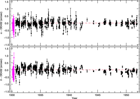
Figure 4. Comparison to DE432. The astrometry from the Lampland plates relative to DE432 is plotted as a function of time. The dashed red curve shows zero. These residuals and the offsets from DE430 shown in Figure 2 are very similar. The points for the 1930 apparition (magenta) were not used in the fit.
Download figure:
Standard image High-resolution imageNote that some of the Pulkovo observations have been re-reduced against the UCAC4 catalog (Khrutskaya et al. 2013). These re-reduced observations from Pulkovo show a slight bias in R.A. relative to the older FK5-based reduction and against the Lampland observations. A misinterpretation of measurement times is one possible cause of such an offset. An advantage of the data reduced against the FK5 catalog is that the measurements were reported as differences relative to a previous JPL ephemeris, DE200. These differences are insensitive to interpretations of measurement times, so the FK5-based reduction is used for this estimation.
The measurement uncertainties assigned to each data set strongly affect the final orbit estimation. The measurement uncertainties used here have been derived from examination of the measurement residuals and by comparing estimates and uncertainties for various data subsets as described in the next section. For the re-reduced data from Lowell Observatory, the measurement uncertainties provided in Table 1 reflect only the random errors for Pluto. Clearly these measurements also contain uncertainties due to the supporting catalog itself. The UCAC4 catalog is based on the system set up by the Tycho-2 star catalog and we assume the catalog errors just pass through to the Pluto measurements. Høg et al. (2000) estimate the errors in the Tycho-2 catalog to have a mean positional error of 60 mas and a mean proper motion error of 2.5 mas year−1. The mean epoch of Tycho-2 is 1991.5 and extrapolating the catalog error to 1940 indicates a position error of 125 mas due to proper motion error. Combining these two components yields a final catalog error contribution of 140 mas which should be added in quadrature to the Pluto measurement uncertainties. This adjustment to the uncertainties makes the data consistent with the residuals from the fit. The Pulkovo measurement uncertainties of 0 2 in R.A. and 03 in decl. are based on the rms of the measurement residuals. The USNO/Flagstaff measurement uncertainties are set to 01, a value that is comparable to the rms of their residuals.
The Pico dos Dias observers provided measurement uncertainties for each observation, taking into account instrument, atmospheric, and star catalog components. However, their data set includes many nights with large numbers of measurements in each night. The reported measurement uncertainties assume that the star catalog errors average down for multiple measurements in a given night. For this fit, it is assumed that the star catalog errors do not average down for multiple measurements in a single night, since the stars closest to Pluto will be the same throughout the night and their position errors should eventually dominate. Therefore the Pico dos Dias measurement uncertainties used in this fit are the error estimate supplied multiplied by the square-root of the number of measurements in the night each measurement was taken.
There are typically four measurements in most nights from Table Mountain, so the measurement uncertainties used of 01 are about twice the observed rms of the measurement residuals to account for multiple measurements per night. The occultation measurement uncertainties used were the rms of their residuals, which are 006 in R.A. and 003 in decl. The mean of the occultation measurement residuals is not quite zero, which affects the observed rms.
The residuals for the measurements after DE432 ephemeris fit appear very similar to the residuals to the DE430 ephemeris (Folkner et al. 2014) so they are not shown here. The residuals for the re-reduced Lowell Observatory measurements are shown in Figure 4 and the yearly summaries are provided in Table 2. Note that the observations from the discovery apparition, described in detail in Section 4.1, were excluded from the fit. The difference between these post-fit residuals and the offsets from DE430 is very small.
Figure 5 shows the difference in the estimated orbit of Pluto from DE432 with the earlier ephemerides DE430 and DE418. Over this time span, the ephemerides all agree to better than 4000 km and at 2015 the differences are less than 2000 km. Also evident is that DE430 is the most similar to DE432 but that is largely a consequence of the constraining data being more similar. The difference between DE432 and DE430 is primarily due to the addition of the re-reduced data from Lowell Observatory. The earlier DE418 estimate included a number of data sets reduced against EME1950 star catalogs which were not used for the estimates of DE430 or DE432. The differences in R.A. and distance to Pluto are consistent with the estimated uncertainty in the Pluto orbit from DE418. The differences in decl. are larger than the estimated uncertainty from DE418. The decl. estimate is more sensitive to tropospheric effects than are R.A. and distance estimates. It is possible that some systematic effect from the troposphere, such as differential color refraction of the troposphere, is not accounted for by the rms of the measurement residuals.

Figure 5. Comparison of DE418 and DE430 to DE432. The difference of DE418-DE432 and DE430-DE432 for Pluto are plotted as a function of time. The dashed red curve shows zero. The top panel is the R.A. difference multiplied by distance. The middle panel is the decl. difference multiplied by distance. The bottom panel is the heliocentric distance difference. All quantities are in kilometers and the plot range is held fixed for all three plots.
Download figure:
Standard image High-resolution imageThe estimated orbit for DE432 is considered stable and repeatable, and agrees well with estimates based on independent data subsets. Also, importantly, the re-reduced data from Lowell Observatory provide good consistency with orbit estimates made without those data included.
4.2.2. Pluto Orbit Uncertainty Estimation
In order to assess the appropriate measurement uncertainties and the accuracy of the estimated orbit of Pluto, the data were divided into four subsets. The re-reduced Lampland data (L), covering 1930–1951, and the Pulkovo data, covering 1930–1992 (P) were the two data sets used with measurements prior to 1990. The data from USNO/Flagstaff combined with Table Mountain and stellar occultation data were used as one set (N) of data since 1995 while the measurements from Pico dos Dias (B, for Brazil) were used as a second post-1995 data set. Four combinations of one pre-1990 data set and one post-1995 data set were used to generate four estimates of the orbit of Pluto. These allowed taking the difference for two pairs of estimated orbits with independent data: Lampland/Lowell combined with USNO/TMO/occultation (LN) compared with Pulkovo combined with Pico dos Dias (PB); and Lampland/Lowell combined with Pico dos Dias (LB) compared with Pulkovo combined with USNO/TMO/occultation (PN). Figure 6 shows the differences in estimated orbits of Pluto between those two pairs of independent data sets. In these plots we see that the differences between these independent orbit estimates are less than 3000 km. The range and variations of the differences shown give an indication of the degree of consistency in the orbit estimates and give us more confidence that there are no large sources of unrecognized systematic errors.
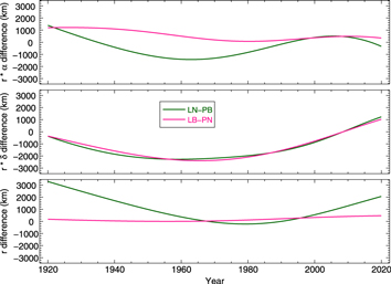
Figure 6. Ephemeris position differences between independent orbit estimates. The top panel is the R.A. difference multiplied by distance. The middle panel is the decl. difference multiplied by distance. The bottom panel is the heliocentric distance difference. All quantities are in kilometers and the plot range is held fixed for all three plots. Two pairs are plotted. L refers to the Lampland data. N refers to data from USNOFS and Table Mountain. P refers to the Pulkovo data. B refers to the Pico dos Dias data (Brazil). The pairs of initials, eg. LN, indicate those two datasets were used to generate an ephemeris.
Download figure:
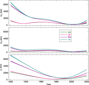
Standard image High-resolution imageFigure 7 shows the estimated uncertainties in each of the four orbit estimates based on the measurement uncertainties used. The estimated uncertainties shown are a factor of two times the formal estimated uncertainties. The factor of two was applied so that the differences in estimated R.A. and distance to Pluto were comparable with the uncertainties. It is common for formal uncertainties to underestimate actual uncertainty since measurements are usually assumed to be uncorrelated in the orbit estimation process when in fact many measurements may share common unmodeled errors, such as star catalog zone errors.
Figure 7. Uncertainties for data subset fits. The top panel is the R.A. uncertainty multiplied by distance ( ). The middle panel is the decl. uncertainty multiplied by distance (
 ). The bottom panel is the heliocentric distance uncertainty (
 ). All quantitites are in kilometers and the plot range is held fixed for all three plots. Four individual fits are plotted. L refers to the Lampland data. N refers to data from USNOFS and Table Mountain. P refers to the Pulkovo data. B refers to the Pico dos Dias data (Brazil). Each line thus represents the uncertainty from fits to two out of the four available datasets.
Download figure:
Standard image High-resolution image
It can be seen in Figures 6 and 7 that the Lampland measurements, with the assumed measurement uncertainties, provide the strongest information on the long-term R.A. estimate and on estimated distance. The two combinations including the Lampland data, with either the USNO/TMO/occultations or with the Pico Dos Dias data, provide uncertainties in R.A. and distance that are similar to each other and with smaller estimated uncertainty than the combinations including the Pulkovo data. These results show the uncertainty on Plutoʼs heliocentric distance at the time of the New Horizons encounter in 2015 is roughly 1000 km. Work continues to refine this determination and its uncertainty but this result already demonstrates the ephemeris is good enough to support the mission design for the flyby.
4.3. Implications for New Horizons
Ultimately, what matters for the New Horizons flyby is that the position of Pluto is known relative to the spacecraft trajectory. This position comes from JPL in the form of their developmental ephemerides and these ephemerides are improved over time as more data are added. The last such released ephemeris that does not contain the data in this work is DE430. For the purposes of inter-comparing ephemerides, Table 3 contains the position of the Pluto-system barycenter with respect to the Sun at TDB 2015 July 15 12:00:00 (no light-time) after subtracting this position as computed with DE430. We have also included selected ephemerides from independent analyses (though much of the data is in common throughout). The trend in the position is obvious and the more recent values being smaller is consistent with an ephemeris that is improving with time. The Lampland data allow an improvement in the Pluto ephemeris uncertainty. The resulting estimate is consistent with JPL ephemerides starting with DE418 when the Pulkovo data set was included and dominated the pre-1990 measurement data sets. The Lampland data are consistent with the Pulkovo data, and comparisons of Pluto orbit estimates with independent data sets show that the orbit estimates and their associated uncertainties are robust. A final comparison between EPM2014a (Pitjeva & Pitjeva 2014) and DE432 show the heliocentric distances at the time of encounter agree to 325 km.
Table 3. Ephemeris Comparison to DE430
| Ephemeris | Release Date |

|

|

|

|
Notes |
| (km) | (km) | (km) | (km) | |||
| INPOP13c | 2014-Jun-25 | 1961 | 586 | 665 | 2152 | Verma et al. (2014) |
| DE432 | 2014-May-01 | −107 | 1046 | −366 | 1048 | Lampland data added |
| EPM2014a | 2014-Apr-29 | −737 | −1664 | −143 | 1380 | Pitjeva & Pitjeva (2014) |
| DE430 | 2013-Mar-25 | 0. | 0. | 0. | 0. | Added Pico Dos Dias, Assafin et al. occultations |
| EPM11 | 2012-Dec-20 | −115 | −1963 | −671 | 2014 | Pitjeva (2013) |
| ODIN | 2012-Oct-29 | 295 | −4992 | −170 | 4639 | Beauvalet et al. (2013) |
| DE425 | 2012-May-09 | 290 | 1124 | 412 | −1091 | Added new Mars data |
| DE424 | 2011-Sep-14 | 287 | 1124 | 417 | −1093 | Added 2011 USNOFS & TMO data |
| DE423 | 2010-Feb-10 | 152 | 169 | 163 | −173 | Added 2010 USNOFS & TMO data |
| DE422 | 2009-Sep-29 | 78 | 1509 | 271 | −1440 | Dropped AGC, added USNOFS & TMO through 2009 |
| INPOP08 | 2009-Aug-24 | −2838 | 4465 | 1189 | −5142 | Fienga et al. (2009) |
| EPM08 | 2008-Apr-01 | −333 | 94 | −1281 | 289 | Pitjeva (2010) |
| DE421 | 2008-Mar-31 | −163 | 33 | −1287 | 388 | New Mars and Lunar data |
| DE418 | 2007-Aug-02 | −214 | 964 | −1296 | −462 | Added Pulkovo data (Rylkov et al.) |
| DE414 | 2006-Apr-21 | 927 | 10444 | 542 | −9394 | ⋯ |
| DE413 | 2004-Nov-04 | 1250 | 11522 | 1001 | −10452 | ⋯ |
| EPM2004 | 2004-Oct-07 | −850 | −1183 | −2623 | 1792 | Pitjeva (2005) |
| DE405 | 1998-Aug-26 | 1938 | 12129 | 2947 | −11523 | ⋯ |
| DE403 | 1995-May-22 | −5726 | 2381 | −3607 | −2262 | ⋯ |
| DE202 | 1987-Oct-31 | −55783 | −71415 | −17442 | 57085 | ⋯ |
| DE200 | 1982-May-18 | −133878 | −132731 | −15421 | 92654 | ⋯ |
Note. Offsets are computed for the Pluto system barycenter with respect to the Sun at TDB 2015-Jul-15 12:00:00, no light-time correction, ephemeris—DE430. Comments, where supplied, indicate changes to that ephemeris compared to the previous within the same family. See text for additional details.
Download table as: ASCIITypeset image
5. CONCLUSIONS
We presented a new analysis of historical photographic plates based on new star catalogs and in so doing provide significant new constraints on the orbit of Pluto. These data are archived at Lowell Observatory along with all the digital information in case of future analyses with even better star catalogs. These new data, when combined with other large high-quality data sets permit making independent orbit determinations that guard against unrecognized systematic errors. The newest ephemeris, DE432, has the best yet estimate for the orbit of Pluto and with an uncertainty of ∼1000 km is of sufficient quality to support the impending flyby of New Horizons in 2015. Given that Pluto has still not completed a full orbit since discovery, the need for continued high-quality astrometric observations continues.
This work would not have been possible without the tireless dedication of Carl Lampland and the subsequent attitude of preserving old data by H. Giclas and Lowell Observatory. Support from New Horizons was essential in completing this work with special thanks to J. Cook, C. Conrad, and C. Olkin. We are grateful for the efforts of J. Grindlay, R. (Bob) Simcoe, E. Los, A. Doane, R. Teague, S. Siok, and R. Kenison for the use of DASCH and assistance with scanning. Thanks also to the Royal Observatory of Belgium and Jean-Pierre DeCuyper and Veronique Dehant as well as Norbert Zacharias for their assistance in earlier testing efforts. Thanks to R. F. Poppen for many algorithmic insights pertaining to digital image processing (e.g., findsrc.pro, basphote.pro). Those contributions were made more than 30 years ago and are still extremely useful and valuable. The research described in this paper was in part carried out at the Jet Propulsion Laboratory, California Institute of Technology, under a contract with the National Aeronautics and Space Administration.
Footnotes
- 3
This routine and others mentioned in this paper are publicly available at http://www.boulder.swri.edu/~buie/idl.