


ABSTRACT
The use of type Ic super luminous supernovae (SLSNe Ic) to examine the cosmological expansion introduces a new standard ruler with which to test theoretical models. The sample suitable for this kind of work now includes 11 SLSNe Ic, which have thus far been used solely in tests involving the Λ cold dark matter (ΛCDM) model. In this paper, we broaden the base of support for this new, important cosmic probe by using these observations to carry out a one-on-one comparison between the and ΛCDM cosmologies. We individually optimize the parameters in each cosmological model by minimizing the statistic. We also carry out Monte Carlo simulations based on these current SLSNe Ic measurements to estimate how large the sample would have to be in order to rule out either model at a ∼99.7% confidence level. The currently available sample indicates a likelihood of ∼70–80% that the universe is the correct cosmology versus ∼20–30% for the standard model. These results are suggestive, though not yet compelling, given the current limited number of SLSNe Ic. We find that if the real cosmology is ΛCDM, a sample of ∼240 SLSNe Ic would be sufficient to rule out at this level of confidence, while ∼480 SLSNe Ic would be required to rule out ΛCDM if the real universe is instead . This difference in required sample size reflects the greater number of free parameters available to fit the data with ΛCDM. If such SLSNe Ic are commonly detected in the future, they could be a powerful tool for constraining the dark-energy equation of state in ΛCDM, and differentiating between this model and the universe.


1. INTRODUCTION
A new type of luminous transient has been identified in recent years through the use of deep, wide surveys searching for supernovae in the local universe (Quimby et al. 2005, 2007; Quimby 2006; Smith et al. 2007; Drake et al. 2009; Rau et al. 2009; Kaiser et al. 2010; Gal-Yam 2012; Baltay et al. 2013). These super luminous supernovae (SLSNe) have peak magnitudes mag and integrated burst energies erg. They are therefore much brighter than both Type Ia SNe (SNe Ia) and the majority of core-collapse events. Their unusually high peak luminosities, hot blackbody temperatures, and bright rest frame ultraviolet emission (which renders their continuum easily detectable at optical and near-infrared wavelengths at high redshifts; Cooke et al. 2012) allow them to be studied in concert with possible gamma-ray burst (GRB) associations (Cano & Jakobsson 2014; Li et al. 2014) and, more importantly, make them viable standardizable candles and distance indicators for use as cosmological probes (Inserra & Smartt 2014).


Inserra et al. (2013) and Nicholl et al. (2013) used the classification term SLSNe Ic to refer to all the hydrogen poor SNLSe, though there appear to be at least two observational groups in this category. These are distinguished via the terms SN2005ap-like and SN2007bi-like events, since these are the prototypes with the faster and slower evolving light curves. SLSNe Ic have now been discovered out to redshifts z ∼ 4 (Chomiuk et al. 2011; Berger et al. 2012; Cooke et al. 2012; Howell et al. 2013), and appear to be rather homogeneous in their spectroscopic and photometric properties.
The brighter events decline more slowly, not unlike the Phillips relation for SNe Ia, which raises the possibility of correlating their peak magnitudes to their decline over a fixed number of days to reduce the scatter (Rust 1974; Pskovskii 1977; Phillips 1993; Hamuy et al. 1996). Without the use of such a relation, the uncorrected raw mean magnitudes show a dispersion of ∼0.4 (e.g., Inserra & Smartt 2014). Correlating the peak magnitude to the decline over 30 days reduces the scatter in standardized peak magnitudes to ±0.22 mag. And apparently using a magnitude–color evolution reduces this scatter even more, to a low value somewhere between ±0.08 and ±0.13 mag.
It is therefore quite evident that SLSNe Ic may be useful cosmological probes, perhaps even out to redshifts much greater () than those accessible using SNe Ia. The currently available sample, however, is still quite small; adequate data to extract correlations between empirical, observable quantities, such as light curve shape, color evolution and peak luminosity, are available only for tens of events. Our focus in this paper is specifically to study whether SLSNe Ic can be used—not only to optimize the parameters in the Λ cold dark matter (ΛCDM) model (Cano & Jakobsson 2014; Inserra & Smartt 2014; Li et al. 2014), e.g., to refine the dark-energy equation of state but, also—to carry out comparative studies between competing cosmologies, such as ΛCDM versus the universe (Melia 2007, 2013a; Melia & Abdelqader 2009; Melia & Shevchuk 2012).


Like ΛCDM, the universe is a Friedmann–Robertson–Walker cosmology that assumes the presence of dark energy, as well as matter and radiation. The principle difference between them is that the latter is also constrained by the equation of state , in terms of the total pressure p and energy density ρ. In recent years, this model has generated some discussion concerning its fundamental basis, including claims that it is actually a vacuum solution, even though . However, all criticisms leveled against thus far appear to be based on incorrect assumptions and theoretical errors. A full accounting of this discussion may be found in Melia (2015) and references cited therein.


In fact, the application of model selection tools in one-on-one comparisons between these two cosmologies has shown that the data tend to favor over ΛCDM. Tests completed thus far include high-z quasars (Melia 2013b, 2014), GRBs (Wei et al. 2013), the use of cosmic chronometers (Melia & Maier 2013) and, most recently, the SNe Ia themselves (Wei et al. 2015). In all of these tests, information criteria show that , with the important additional constraint on its equation of state, is favored over ΛCDM with a likelihood of ∼90% versus only ∼10%.


Here, we broaden the comparison between and ΛCDM by now including SLSNe Ic in this study. In Section 2 we briefly describe the currently available sample and our method of analysis. Our results are presented in Section 3. We will find that the current catalog of SLSNe Ic suitable for this study already confirms the tendencies discussed above, though the statistics are not yet good enough to strongly differentiate between these two competing models. We show in Section 4 how large the source catalog needs to be in order to rule out one or the other expansion scenario at a 3σ confidence level, and we present our conclusions in Section 5.

2. METHODOLOGY
Eleven of the SLSNe Ic identified by Inserra & Smartt (2014) are appropriate for this work, and we base our analysis on the methodology described in their paper and in Li et al. (2014). Briefly, the chosen SLSNe Ic must have well sampled light-curves around peak luminosity, and photometric coverage from several days pre-maximum to 30 days (in the rest frame) after the peak. This time delay appears to be optimal for use in the Phillips-like peak magnitude–decline relation (Inserra & Smartt 2014).
All 11 of these events appear to be similar to the well-observed SN2010gx, and these decay rapidly after peak brightness. They belong to the group of 2005ap-like events, the first such SN discovered in this category. Other SLSNe Ic could not be included simply because of lack of sufficient temporal coverage, even though their identification has been securely classified in previous work (see, e.g., Chomiuk et al. 2011; Quimby et al. 2011; Berger et al. 2012; Leloudas et al. 2012; Inserra et al. 2013; Nicholl et al. 2014).
The SNe listed in Table 1 were located in faint, dwarf galaxies, and were unlikely to have suffered significant extinction beyond the reddening induced by interstellar dust in our Galaxy. We here adopt the reddening corrections from Tables 1 and 2 of Inserra & Smartt (2014), who assumed a standard reddening curve with . We also adopt their K-corrections and time dilation effects in order to obtain the absolute rest-frame peak magnitudes. This step is necessary due to the large () redshift coverage of the sample. These are listed in the table, along with the source names, their redshifts, apparent peak magnitudes (and filters), the magnitude decrease over 30 days, and the color change between the 400 and 520 nm synthetic (restframe) bands at peak and 30 days later.


Table 1. Sample of SLSNe Ic
| SN | z | mf | Filter | Af | References | |||||
|---|---|---|---|---|---|---|---|---|---|---|
| SN2011ke | 0.143 | 0.01 | 17.70 (g) | 0.05 | −0.18 | 17.83 ± 0.20 | 2.47 ± 0.16 | 0.54 ± 0.17 | 1, 8 | |
| SN2012il | 0.175 | 0.02 | 18.00 (g) | 0.09 | −0.18 | 18.09 ± 0.21 | 2.19 ± 0.16 | 0.49 ± 0.17 | 1, 8 | |
| PTF11rks | 0.190 | 0.04 | 19.13 (g) | 0.17 | −0.19 | 19.15 ± 0.20 | 2.62 ± 0.14 | 0.95 ± 0.14 | 1, 8 | |
| SN2010gx | 0.230 | 0.04 | 18.43 (g) | 0.13 | −0.23 | 18.53 ± 0.18 | 2.00 ± 0.19 | 0.34 ± 0.16 | 2, 8 | |
| SN2011kf | 0.245 | 0.02 | 18.60 (g) | 0.09 | −0.13 | 18.64 ± 0.18 | 1.49 ± 0.16 | ... | 1, 8 | |
| LSQ12dlf | 0.255 | 0.01 | 18.78 (V) | 0.03 | −0.27 | 19.02 ± 0.12 | 1.00 ± 0.10 | 0.29 ± 0.12 | 3, 8 | |
| PTF09cnd | 0.258 | 0.03 | 18.29 (R) | 0.05 | −0.34 | 18.58 ± 0.22 | 1.09 ± 0.14 | ... | 4, 8 | |
| SN2013dg | 0.265 | 0.01 | 19.06 (g) | 0.03 | −0.30 | 19.33 ± 0.20 | 2.08 ± 0.20 | 0.51 ± 0.17 | 3, 8 | |
| PS1-10bzj | 0.650 | 0.01 | 21.23 (r) | 0.02 | −0.58 | 21.79 ± 0.20 | 1.70 ± 0.14 | 0.60 ± 0.15 | 5, 8 | |
| PS1-10ky | 0.956 | 0.03 | 21.15 (i) | 0.06 | −0.73 | 21.82 ± 0.18 | 1.31 ± 0.15 | 0.30 ± 0.18 | 6, 8 | |
| SCP-06F6 | 1.189 | 0.01 | 21.04 (z) | 0.01 | −1.35 | 22.38 ± 0.20 | 0.89 ± 0.15 | ... | 7, 8 |


Notes. All values are from Inserra & Smartt (2014), except for , which is calculated here. The error bars are directly from Figures 5 and 6 in Inserra & Smartt (2014). Columns: SN name; measured redshift; extinction; observed peak magnitude (AB system) and filter; Galactic extinction in the observed filter; calculation of the synthetic 400 nm magnitude from the observed filter; apparent magnitude mapped into the 400 nm passband, and its dispersion; magnitude decrease in 30 restframe days and its dispersion; the color change between the 400 and 520 nm synthetic bands at peak and 30 days later, and its dispersion.

References. (1) Inserra et al. (2013), (2) Pastorello et al. (2010), (3) Nicholl et al. (2014), (4) Quimby et al. (2011), (5) Lunnan et al. (2013), (6) Chomiuk et al. (2011), (7) Barbary et al. (2009), (8) Inserra & Smartt (2014).
Download table as: ASCIITypeset image
In order to provide consistent, standarized comparative rest frame properties, the observed apparent magnitudes (m in Table 1) have been converted into defined, synthetic magnitudes. Since the SLSNe Ic spectrum around 400 nm is continuum dominated, Inserra & Smartt (2014) defined a synthetic passband with an effective width of 80 nm, centered at wavelength 400 nm, having steep wings and a flat top. In Table 1, this is referred to as the 400 nm band. All of the chosen events in this table have sufficient photometric coverage to allow the K-correction to uniformly map the observed filter's wavelength range to this 400 nm bandpass in the rest frame. The absolute magnitudes are then formally defined by the relation

where is the apparent magnitude mapped into the restframe 400 nm band, μ is the distance modulus calculated from the luminosity distance, mf is the AB magnitude in the observed filter f (g, V, R, r, z, or i, as indicated in Table 1), is the Galactic extinction in the observed filter, and is the K-correction from the observed filter in Table 1 to the synthetic 400 nm bandpass. The values of and m(400) are listed in Table 1. Note that m(400) is a cosmology-independent apparent magnitude.


The peak magnitude–decline relation for SLSNe Ic in the rest frame 400 nm band is (Inserra & Smartt 2014)

where α is the slope, is the decline at 30 days, and M0 is a constant representing the absolute peak magnitude at . Inserra & Smartt (2014) also found that Mpeak(400) appears to have a strong color dependence. Redder objects are fainter and also become redder faster. This peak magnitude–color evolution relation is given by


where is the difference in color M(400)–M(520) between the peak and 30 days later. (Note that M0 and α need not be the same in these two expressions.)

With Equations (2) and (3), an effective (standardized) apparent magnitude meff may be obtained as follows:

The term represents an adjustment due to the peak magnitude–decline relation, in terms of , or the peak magnitude–color evolution relation, in terms of , as the case may be. The effective apparent magnitude may also be expressed as (Perlmutter et al. 1997, 1999)


where H0 is the Hubble constant in units of km s−1 Mpc−1 and dL is the luminosity distance in units of Mpc. Here Υ is the "H0-free" 400 nm absolute peak magnitude, represented in terms of the standardizable absolute magnitude M0, according to the definition

(see Li et al. 2014 and references cited therein).
The apparent correlations suggest the use of two "nuisance" parameters (α and Υ) whose optimization along with the model parameters decreases the overall scatter in the distance modulus. For each model, we therefore find the best fit by minimizing the statistic, defined as follows:


In ΛCDM, the luminosity distance depends on several parameters, including H0 and the mass fractions , , and , defined in terms of the current matter (), radiation (), and dark-energy () densities, and the critical density . Assuming zero spatial curvature, so that , the luminosity distance to redshift z is given by the expression


where is the dark-energy equation of state. The Hubble constant H0 cancels out in Equation (7) when we multiply dL by H0, so the essential remaining parameters in flat ΛCDM are and . If we further assume that dark energy is a cosmological constant with , then only the parameter is available to fit the data.


In the universe (Melia 2007; Melia & Abdelqader 2009; Melia & Shevchuk 2012), the luminosity distance depends only on H0, but since here too the Hubble constant cancels out in the product , there are actually no free (model) parameters left to fit the SLSNe Ic data. In this cosmology,


3. RESULTS
We have assumed that SLSNe Ic can be used as standardizable candles and applied the decline relation (with 11 objects) and the peak magnitude–color evolution relation (with eight objects) to compare the standard (ΛCDM) model with the Rh = ct universe. In this section, we discuss how the fits have been optimized, first for ΛCDM, and then for Rh = ct. The outcome for each model is more fully described and discussed in subsequent sections.

3.1. ΛCDM
In the most basic ΛCDM model, the dark-energy equation of state parameter, wde, is exactly −1. The Hubble constant H0 cancels out in Equation (7) when we multiply dL by H0, so the essential remaining parameter is . SN Ia measurements (see, e.g., Perlmutter et al. 1998, 1999; Riess et al. 1998; Schmidt et al. 1998), cosmic microwave background anisotropy data (e.g., Hinshaw et al. 2013), and baryon acoustic oscillation peak length scale estimates (e.g., Samushia & Ratra 2009), strongly suggest that we live in a spatially flat, dark energy-dominated universe with concordance parameter values and km s−1 Mpc−1.


We will therefore first attempt to fit the data with this concordance model, using prior values for all the model parameters, but not the two "nuisance" parameters α and Υ. For the decline relation (with 11 objects), the resulting constraints on α and Υ are shown in Figure 1(a). For this fit, we obtain , , and a per degree of freedom of , remembering that all of the ΛCDM parameters are assumed to have prior values, except for the "nuisance" parameters α and Υ. (The corresponding data and best fit are shown in the top left-hand panel of Figure 4.) For the peak magnitude–color evolution relation (with eight objects), the resulting constraints on α and Υ are shown in Figure 1(b). The best-fit parameters are , . The per degree of freedom for the concordance model with these optimized "nuisance" parameters is (see also the top right-hand panel in Figure 4).


Figure 1. 1–3σ constraints on α and Υ for the concordance model, using the decline relation (panel (a)) and the peak magnitude–color evolution relation (panel (b)).

Download figure:
Standard image High-resolution imageIf we relax some of the priors, and allow to be a free parameter, we obtain the 1– constraint contours shown in the top panel of Figure 2 for the decline relation, and the bottom panel for the peak magnitude–color evolution relation. These contours show that at the 1σ level, the optimized parameter values are , , and . We find that the per degree of freedom for the optimized flat ΛCDM model is . The bottom panel of Figure 2 shows the 1– constraints on α, Υ, and for the flat ΛCDM model, using the peak magnitude–color evolution relation. The contours show that at the 1σ-level, , , but that is poorly constrained; only a lower limit of ∼0.05 can be set at this confidence level and the best-fit is 0.59. The per degree of freedom is .


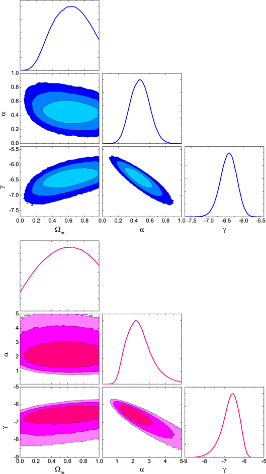
Figure 2. Top panel: constraints on α, Υ, and for the flat ΛCDM model, using the decline relation. Bottom panel: same as the top panel, but using the peak magnitude–color evolution relation.


Download figure:
Standard image High-resolution image3.2. The Universe

The Rh = ct universe has only one free parameter, , but since the Hubble constant cancels out in the product , there are actually no free (model) parameters left to fit the SLSNe Ic data. The results of fitting the ΔM30 decline relation with this cosmology are shown in Figure 3(a). We see here that the best fit corresponds to and . With degrees of freedom, the reduced is . The results of fitting the peak magnitude–color evolution relation with this cosmology are shown in Figure 3(b). We see here that the best fit corresponds to and . With degrees of freedom, the reduced is .


Figure 3. 1– constraints on α and Υ for the universe, using the decline relation (panel (a)) and the peak magnitude–color evolution relation (panel (b)).


Download figure:
Standard image High-resolution imageTo facilitate a direct comparison between ΛCDM and Rh = ct, we show in Figure 4 the Hubble diagrams for SLSNe Ic. In the left panel of Figure 4, the effective magnitudes meff of 11 SLSNe Ic are plotted as solid points, together with the best-fit theoretical curves (from top to bottom) for the concordance model (with prior values of the parameters, and with and ), for the optimized flat ΛCDM model (with , and with , and ). and for the universe (with and ). The Hubble diagrams derived using the peak magnitude–color evolution relation are shown in the right-hand panels of Figure 4. Here, the effective magnitudes meff of 8 SLSNe Ic are plotted as solid points, together with the best-fit theoretical curves for the concordance model (with prior values of the parameters, and with α = 2.00 and ), for the optimized flat ΛCDM model (with , and with , and ), and for the Rh = ct universe (with and ). Strictly based on their values, the optimized ΛCDM model and the Rh = ct universe appear to fit the SLSNe Ic data comparably well. However, because these models formulate their observables (such as the luminosity distances in Equations(8) and (9) differently, and because they do not have the same number of free parameters, a comparison of the likelihoods for either being closer to the "true" model must be based on model selection tools.


Figure 4. Hubble diagrams for SLSNe Ic. The effective apparent magnitudes of SLSNe Ic are plotted as solid points, together with their corresponding best-fit theoretical curves. Left: the effective magnitudes are calculated using the decline relation. Right: the effective magnitudes are calculated using the peak magnitude–color evolution relation.

Download figure:
Standard image High-resolution image3.3. Model Selection Tools
Several information criteria commonly used in cosmology (see, e.g., Melia & Maier 2013, and references cited therein) include the Akaike Information Criterion, , where n is the number of free parameters (Akaike 1973; Takeuchi 2000; Liddle 2004, 2007; Tan & Biswas 2012), the Kullback Information Criterion, (Bhansali & Downham 1977; Cavanaugh 1999, 2004), and the Bayes Information Criterion, , where N is the number of data points (Schwarz 1978; Liddle et al. 2006; Liddle 2007). With characterizing model , the unnormalized confidence that this model is true is the Akaike weight . Model has a likelihood of


of being the correct choice in this one-on-one comparison. The difference determines the extent to which is favored over . For Kullback and Bayes, the likelihoods are defined analogously.


With the optimized fits we have reported in this paper, our analysis of the ΔM30 decline relation (with 11 objects) shows that Rh = ct is favored over the flat ΛCDM model with a likelihood of ≈63.4% versus 36.6% using AIC, ≈74.1% versus ≈25.9% using KIC, and ≈67.9% versus ≈32.1% using BIC. In our one-on-one comparison using the peak magnitude–color evolution relation (with eight objects), the Rh = ct universe is preferred over ΛCDM with a likelihood of ≈72.7% versus 27.3% using AIC, ≈81.5% versus ≈18.5% using KIC, and ≈73.5% versus ≈26.5% using BIC.
4. MONTE CARLO SIMULATIONS WITH A MOCK SAMPLE
These results are interesting, though the current sample of SLSNe Ic is clearly too small for either model to be ruled out just yet. However, this situation will change with the discovery of new SNe, particularly at redshifts . To anticipate how well the SLSNe Ic catalog obeying the peak magnitude–color evolution relation may be used to constrain the dark-energy equation of state in ΛCDM, and to differentiate between this standard model and the Rh = ct universe, we will here produce mock samples of SLSNe Ic based on the current measurement accuracy. In using the model selection tools, the outcome AIC1−AIC2 (and analogously for KIC and BIC) is judged "positive" in the range Δ = 2−6, "strong" for Δ = 6−10, and "very strong" for . In this section, we will estimate the sample size required to significantly strengthen the evidence in favor of Rh = ct or ΛCDM, by conservatively seeking an outcome even beyond , i.e., we will see what is required to produce a likelihood ∼99.7% versus ∼0.3%, corresponding to a 3σ confidence level.


We will consider two cases: one in which the background cosmology is assumed to be ΛCDM, and a second in which it is Rh = ct, and we will attempt to estimate the number of SLSNe Ic required in each case to rule out the alternative (presumably incorrect) model at a ∼99.7% confidence level. The synthetic SLSNe Ic are each characterized by a set of parameters denoted as (z, m[400], ). We generate the synthetic sample using the following procedure.
![${\Delta }{{M}_{30}}[400-520]$](https://content.cld.iop.org/journals/1538-3881/149/5/165/revision1/aj512225ieqn154.gif)
- 1.Since a subclass of broad-lined SNe Ic are observed to be associated with GRBs (Hjorth et al. 2003; Stanek et al. 2003), we simulate the z-distribution of our sample based on the observed z-distribution of GRBs. Shao et al. (2011) found that the z-distribution of GRBs appears to be asymptotic to a parameter-free probability density distribution, . The redshift z of our SLSNe Ic events is generated randomly from this function. Since they can be discovered out to redshifts z ∼ 4 (e.g., Chomiuk et al. 2011; Berger et al. 2012; Cooke et al. 2012; Howell et al. 2013), the range of redshifts for our analysis is [0, 4]. We assign the absolute peak magnitude M(400) uniformly between −23.0 and −21.0 mag, based on the current SLSNe Ic measurements.
- 2.
- 3.With the selected z and M(400) values, we first infer a from the peak magnitude–color evolution relation in a flat ΛCDM cosmology with and km (Section 4.1), or the universe with km (Section 4.2). And then we add scatter to this relation by assigning a dispersion to the value; i.e., we randomly map this quantity to the new value assuming a normal distribution with a center at and a dispersion mag. This value of σ is typical for the current (observed) peak magnitude–color evolution relation, which yields a standard deviation mag for the linear fit (Inserra & Smartt 2014). If mag, this SLSNe Ic is included in our sample. Otherwise, it is excluded.
- 4.We next assign "observational" errors to and . We will assign a dispersion to each event i, where ki is a random number between 0 and 1.


This sequence of steps is repeated for each new SLSNe Ic in the sample, until we reach the likelihood criterion discussed above. As with the real 11-SLSNe Ic sample, we optimize the model fits by minimizing the function in Equation (7).

4.1. Assuming ΛCDM as the Background Cosmology
We have found that a sample of at least 240 SLSNe Ic is required in order to rule out at the ∼99.7 % confidence level. The optimized parameters corresponding to the best-fit wCDM model for these simulated data are displayed in Figure 5. To allow for the greatest flexibility in this fit, we relax the assumption that dark energy is a cosmological constant with , and allow to be a free parameter, along with . Figure 5 shows the 1D probability distribution for each parameter (, , α, Υ), and 2D plots of the 1– confidence regions for two-parameter combinations. The best-fit values for wCDM using the simulated sample with 240 SNe in the ΛCDM model are , , , and .


Figure 5. 1D probability distributions and 2D regions with the 1– contours corresponding to the parameters , , α, and Υ in the best-fit wCDM model, using the simulated sample with 240 SLSNe Ic, assuming ΛCDM as the background cosmology.


Download figure:
Standard image High-resolution imageTo gauge the impact of these constraints more clearly, we show in Figure 6 the confidence regions (shaded, with red contours) for and using these 240 simulated SLSNe Ic (the same as the bottom left-hand panel of Figure 5), and compare these to the constraint contours for the 580 Union2.1 Type Ia SN data (Suzuki et al. 2012) (represented by the blue contours in Figure 6). It is straightforward to see how effectively the SLSNe Ic could be used as a cosmological tool, because the confidence regions resulting from their analysis are smaller (and narrower for ) than those corresponding to the Type Ia events. The better constraints are mainly due to the fact that SLSNe Ic are distributed over a much wider redshift range, extending toward high-z, where tighter constraints on the model can be achieved.


Figure 6. 1σ, 2σ, and 3σ confidence regions for the wCDM model using simulated SLSNe Ic (shaded, with red contours), compared with those (dashed blue contours) associated with the 580 Union2.1 Type Ia SNe.
Download figure:
Standard image High-resolution imageIn Figure 7, we show the corresponding 2D contours in the α–Υ plane for the universe. The best-fit values for the simulated sample are and .


Figure 7. 2D region with the 1– contours for the parameters α and Υ in the universe, using a sample of 240 SLSNe Ic, simulated with ΛCDM as the background cosmology. The simulated model parameters were , , and km s−1 Mpc−1.


Download figure:
Standard image High-resolution imageSince the number N of data points in the sample is now much greater than one, the most appropriate information criterion to use is the BIC. The logarithmic penalty in this model selection tool strongly suppresses overfitting if N is large (the situation we have here, which is deep in the asymptotic regime). With N = 240, our analysis of the simulated sample shows that the BIC would favor the wCDM model over by an overwhelming likelihood of versus only (i.e., the prescribed confidence limit).


4.2. Assuming as the Background Cosmology

In this case, we assume that the background cosmology is the universe, and seek the minimum sample size to rule out wCDM at the confidence level. We have found that a minimum of 480 SLSNe Ic are required to achieve this goal. To allow for the greatest flexibility in the wCDM fit, here too we relax the assumption of dark energy as a cosmological constant with , and allow to be a free parameter, along with . In Figure 8, we show the 1D probability distribution for each parameter (, , α, Υ), and 2D plots of the 1– confidence regions for two-parameter combinations. The best-fit values for wCDM using this simulated sample with 480 SLSNe Ic are , , , and . Note that the simulated SLSNe Ic give a good constraint on , but a weak constraint on ; only an upper limit of 0.09 can be set at the confidence level.


Figure 8. Same as Figure 5, except now with as the (assumed) background cosmology. The simulated model parameter was km s−1 Mpc−1.


Download figure:
Standard image High-resolution imageThe corresponding 2D contours in the α–Υ plane for the universe are shown in Figure 9. The best-fit values for the simulated sample are and . These are similar to those in the standard model, but not exactly the same, reaffirming the importance of reducing the data separately for each model being tested. With N = 480, our analysis of the simulated sample shows that in this case the BIC would favor over wCDM by an overwhelming likelihood of versus only (i.e., the prescribed confidence limit).


Figure 9. Same as Figure 7, except now with as the (assumed) background cosmology.

Download figure:
Standard image High-resolution image5. CONCLUSIONS
It is quite evident that SLSNe Ic may be useful cosmological probes, perhaps even out to redshifts much greater () than those accessible using SNe Ia. The currently available sample, however, is still quite small; adequate data to extract correlations between empirical, observable quantities, such as light curve shape, color evolution and peak luminosity, are available only for tens of events. In this paper, we have proposed to use SLSNe Ic for an actual one-on-one comparison between competing cosmological models. This must be done because the results we have presented here already indicate a strong likelihood of being able to discriminate between models such as ΛCDM and . Such comparisons have already been made using, e.g., cosmic chronometers (Melia & Maier 2013), GRBs (Wei et al. 2013), and SNe Ia (Wei et al. 2015).


We have individually optimized the parameters in each model by minimizing the statistic. With the optimized fits we have reported above, our analysis of the decline relation (with 11 objects) shows that is favored over the flat ΛCDM model with a likelihood of 63–74% versus 26–37% (depending on the information criterion). In our one-on-one comparison using the peak magnitude–color evolution relation (with eight objects), the universe is preferred over ΛCDM with a likelihood of 73–82% versus 18–27%.


But though SLSNe Ic observations currently tend to favor over ΛCDM, the known sample of such measurements is still too small for us to completely rule out either model. We have therefore considered two synthetic samples with characteristics similar to those of the eight known SLSNe Ic measurements, one based on a ΛCDM background cosmology, the other on . From the analysis of these simulated SLSNe Ic, we have estimated that a sample of about 240 such events are necessary to rule out at a ∼99.7% confidence level if the real cosmology is in fact ΛCDM, while a sample of at least 480 SNe would be needed to similarly rule out wCDM if the background cosmology were instead . The difference in required sample size results from wCDM's greater flexibility in fitting the data, since it has a larger number of free parameters.


Our simulations have also shown that a moderate sample size of ∼250 events could reach much tighter constraints on the dark-energy equation of state and on the matter density fraction than are currently available with the 580 Union2.1 Type Ia SNe. If SLSNe Ic can be commonly detected in the future, they have the potential of greatly refining the measurement of cosmological parameters, particularly the dark-energy equation of state .


Assembling samples of this size may be feasible with upcoming surveys. For example, the planned survey SUDSS (Survey Using Decam for Super-luminous Supernovae) using the Dark Energy Camera on the CTIO Blanco 4 m telescope (Inserra & Smartt 2014), and the Subaru/Hyper Suprime-Cam deep survey (Tanaka et al. 2012), have a goal of discovering several hundred SLSNe out to over 3 yr by imaging tens of square degrees to a limiting magnitude ∼25 every 2 weeks. These numbers are based on an estimated production in the local universe by Quimby et al. (2013), who reported a rate of events Gpc−3 yr−1 at a weighted redshift of . This number is low (0.01%) compared to that of SNe Ia. McCrum et al. (2014) estimate a SN Ic rate of the overall core-collapse SN rate within , though this number could be higher at (Cooke et al. 2012) due, perhaps, to a decreasing metallicity. Moreover, the increase in cosmic star formation rate would boost the absolute numbers of SLSNe. As far as observations from the ground are concerned, assembling a sample of several hundred SLSNe Ic over 3–5 yr therefore looks quite promising, particulary with the surveying capability of LSST (see, e.g., Lien & Fields 2009), which should cover the whole sky every 2 nights, down to a limiting magnitude ∼24. The expected rate of discovery of core-collapse SNe with this survey is expected to be ∼1–2 s−1 out to a redshift z ∼ 2. Given that of these are expected to be SNe Ic in this redshift range, one should expect LSST to assemble a ∼500 SLSN sample in less than a year. The situation from space is even more exciting. Detecting SLSNe Ic out to redshifts z ∼10 via their restframe 400 and 520 nm bands is plausible with, e.g., EUCLID (Laureijs et al. 2011), WFIRST and the James Webb Space Telescope (specifically the NIRCam).6


A major problem with this approach right now, however, is that one must rely on the use of a luminosity-limited sample of supernovae, i.e., those selected to be super-luminous with peak magnitudes mag and integrated burst energies ∼ erg (Inserra & Smartt 2014), in order to test the luminosity distances. The difficulty is that the luminosity-limited sample may turn out to be different with different background cosmologies, given that their inferred luminosities are themselves dependent on the models. This situation is unlikely to change as the sample grows, so it would be necessary to find a way of identifying these SNe, other than simply through their magnitudes. Fortunately, in the case of versus ΛCDM, even though their luminosity distances are formulated differently, it turns out that the ensuing distance measures derived from these are quite similar all the way out to z ∼ 6. As such, SLSNe Ic that make the cut for one model and not the other are the exception rather than the rule. In other words, the luminosity-limit applied to the sample examined here does not bias either model very much. But this may not be true in general, and an alternative method of selection is highly desirable.


We are very grateful to Cosimo Inserra for helpful, clarifying discussions, and especially to Stephen Smartt for his thoughtful review of the manuscript, which has led to an improvement in the presentation of our results. This work is partially supported by the National Basic Research Program ("973" Program) of China (Grants 2014CB845800 and 2013CB834900), the National Natural Science Foundation of China (grants Nos. 11322328, 11373068, 11173064, and 11233008), the One-Hundred-Talents Program and the Youth Innovation Promotion Association, and the Strategic Priority Research Program "The Emergence of Cosmological Structures" (Grant No. XDB09000000) of the Chinese Academy of Sciences, and the Natural Science Foundation of Jiangsu Province (grant no.BK2012890). F.M. is also grateful to Amherst College for its support through a John Woodruff Simpson Lectureship, and to Purple Mountain Observatory in Nanjing, China, for its hospitality while this work was being carried out. This work was partially supported by grant 2012T1J0011 from The Chinese Academy of Sciences Visiting Professorships for Senior International Scientists, and grant GDJ20120491013 from the Chinese State Administration of Foreign Experts Affairs.