


ABSTRACT
We present a detailed investigation of the low-amplitude contact binary HI Dra based on the new VRcIc CCD photometric light curves (LCs) combined with published radial velocity (RV) curves. Our completely covered LCs were analyzed using PHOEBE and revealed that HI Dra is an overcontact binary with low fill-out factor f = 24 ± 4(%) and temperature difference between the components of 330 K. Two spotted models are proposed to explain the LC asymmetry, between which the A subtype of W UMa type eclipsing systems, with a cool spot on the less massive and cooler component, proves to be more plausible on evolutionary grounds. The results and stability of the solutions were explored by heuristic scan and parameter perturbation to provide a consistent and reliable set of parameters and their errors. Our photometric modeling and RV curve solution give the following absolute parameters of the hot and cool components, respectively: Mh = 1.72 ± 0.08  and Mc = 0.43 ± 0.02
  , Rh = 1.98 ± 0.03
  and Rc = 1.08 ± 0.02
  , and Lh = 9.6 ± 0.1
  and Lc = 2.4 ± 0.1
  . Based on these results the initial masses of the progenitors (1.11 ± 0.03
  and 2.25 ± 0.07
  , respectively) and a rough estimate of the age of the system of 2.4 Gyr are discussed.
Export citation and abstract BibTeX RIS
1. INTRODUCTION
The most common type of overcontact binary is the W UMa type that has an orbital period between 0.2 and 0.8 days and consists of two main-sequence stars with spectral types ranging from A to K sharing a common convective envelope, thus resulting in a near equalization of the surface temperature with differences not more than a few percent. The W UMa systems are frequently classified either as A types or W types depending on whether the larger or smaller star has the higher temperature (Binnendijk 1970). In A types, the more massive star is eclipsed at primary minimum while the reverse is true for the W types (i.e., the more massive component is the cooler one).
HI Dra (HD 171848 = HIP 90972 = TYC 3917–2301–1 = GSC 03917–02301, αJ2000 = 18h 33m 24 4 and δJ2000 = +58° 42' 23
 4, V = 9.01 mag) was discovered as a variable star by the Hipparcos mission (ESA 1997) with a period of 0.2987090 days and was classified as an RR Lyrae (RRC) variable star (ESA 1997; Kazarovets et al. 1999). The binarity of HI Dra first suggested by Gomez-Forrellad et al. (1999), who performed photometric observations in the V band and classified the system as a β Lyrae or an ellipsoidal binary with a period of 0.597417 days. The authors also noted that both Hipparcos and their new light curves (LCs) show an O'Connell effect of 0.02 mag. Selam (2004) performed a Fourier method on Hipparcos photometric data; extracted the geometric elements: a fill-out factor f = 0.7 (%), mass ratio q = 0.15, and inclination i(°) = 52.5; and suggested a contact binary configuration. The contact configuration of the system was confirmed by Pribulla et al. (2009) based on spectroscopic observations, resulting in a mass ratio q = 0.250 ± 0.005 and a F0-F2V spectral type. The authors noted that the time of the lower conjunction of the more massive component of the system occurs in photometric phase zero, which indicates a W subtype of the W UMa system instead of an A subtype expected from its low mass ratio. Thus, they suggested that either the system's period is changing or the initial epoch determined from Hipparcos photometric data was wrong.
Recently, Rucinski et al. (2013) determined the metallicity of HI Dra to be [M/H] = −0.11 ± 0.14. McDonald et al. (2012), through the construction of the spectral energy distribution of the system from various missions (420–2200 nm), derived its temperature T = 7093 K and luminosity 12.61  . The HI Dra contact binary system is also the primary component of a visual double star discovered by Espin (1905) and listed in the Washington Double Star Catalog (Mason et al. 2014), where the secondary component is a 15th magnitude star separated from HI Dra within 11.4 arcsec. According to the new Hipparcos parallax given by van Leeuwen (2007), it was found that the distance to HI Dra is 255.1 ± 45.6 pc.
These observations show that although there exist the spectroscopic elements of HI Dra, the system is not well studied photometrically or the published LCs are somewhat poorly covered (Hipparcos mission, NSVS1 survey), and the LC asymmetries in the system's maximum light have not yet been considered in detail. Additionally, the times of minima still have not been described. For all these reasons the HI Dra system is interesting for further investigation. In this paper, we present new multi-band LCs and measure the physical properties of the eclipsing system from detailed studies of all available data, such as light and radial velocity (RV) curves.
2. NEW MULTI-BAND CCD PHOTOMETRIC OBSERVATIONS
New multiwavelength CCD photometric observations were carried out on 2011 October 6, 12, and 13 in the V, Ic passbands, on 2012 June 1, 2, 3, and 6 in the VRcIc passbands, and on 2013 October 22 in the Ic passband, with the 35.5 cm f/6.3 Schmidt–Cassegrain telescope at the University of Patras Observatory "Mythodea." This telescope is equipped with an SBIG ST-10 XME CCD camera that has 2184 × 1472 pixels. The size of each pixel is 0 57, resulting in an effective field of view of 20 × 14 arcmin. The standard Johnson–Cousins–Bessel set of BVRcIc was mounted. The typical integration times were 35–55 s for the V band, 30 s for the Rc band, and 40–55 s for the Ic band. Data were processed using the photometry software AIP4WIN (Berry & Burnell 2000) which is based on aperture photometry, including bias and dark subtraction, and flat-field correction. TYC 03917-1556-1 (αJ2000 = 18h33m2313, δJ2000 = 58° 46' 03 7, VT = 9.65 ± 0.03 mag) was used as the comparison star and TYC 3917–2276–1(αJ2000 = 18h32m25064, δJ2000 = 58° 46' 44 96, VT = 10.97 ± 0.08 mag) as the check star. A total of 1363 images was obtained in the three passbands (425 in V, 302 in Rc, and 636 in Ic) and are listed in Table 1 in the form of heliocentric Julian dates (HJD) versus differential magnitudes between the variable star and the comparison (ΔM). The resulting LCs of HI Dra are plotted in Figure 1 as differential magnitudes versus orbital phases; these data were computed according to the ephemeris for our model described in the following section. The resulting photometry accuracy is estimated to be 0.008–0.01 mag.

Figure 1. Observed light curves in the VRcIc bands for HI Dra. Black, blue, and red solid lines denote the synthetic light curves of the unspotted first solution, cool spot Model 1, and hot spot Model 2, respectively. The lower panel displays the residuals for the adopted spotted Model 1.
Download figure:
Standard image High-resolution imageTable 1. VRcIc Observational Data for the Eclipsing Binary HI Dra
| HJD (days) | ΔV (mag) | HJD (days) | ΔRc (mag) | HJD (days) | ΔIc (mag) |
|---|---|---|---|---|---|
| 2456080.32102 | −0.6620 | 2456080.32167 | −0.5880 | 2456081.30956 | −0.5080 |
| 2456080.32399 | −0.6610 | 2456080.32463 | −0.5870 | 2456081.31355 | −0.5130 |
| 2456080.32696 | −0.6610 | 2456080.32760 | −0.5720 | 2456081.31753 | −0.5250 |
| 2456080.32994 | −0.6510 | 2456080.33059 | −0.5750 | 2456081.32151 | −0.5260 |
| 2456080.33292 | −0.6460 | 2456080.33356 | −0.5630 | 2456081.32549 | −0.5470 |
| 2456080.33590 | −0.6340 | 2456080.33654 | −0.5660 | 2456081.32947 | −0.5470 |
| 2456080.33887 | −0.6430 | 2456080.33951 | −0.5690 | 2456081.33345 | −0.5570 |
| 2456080.34183 | −0.6170 | 2456080.34249 | −0.5620 | 2456081.33743 | −0.5530 |
Only a portion of this table is shown here to demonstrate its form and content. Machine-readable and Virtual Observatory (VOT) versions of the full table are available.
Download table as: ASCIITypeset image
3. NEW TIMES OF MINIMUM LIGHT
Our photometric observations include six new weighted times of minimum light observed in V, Rc, and Ic filters. Using the method of Kwee & van Woerden (1956), the times of minima and their errors were determined. In addition to these, all CCD minima have been collected from the literature and added to the times of minima of Nelson.2 Furthermore, using the available time-series data collected during 2007–2008 from the SuperWASP3 database, fifty new times of minima were calculated. Unfortunately, most of them, due to poor photometric accuracy or limited available data points of eclipses, introduced errors of the order of ≥100 s and thus were discarded. The same criterion was applied to poorly determined minima from the literature. All new times of minimum light (6) together with the minima collected from the literature (5) and those calculated from SuperWASP (16) are listed in Table 2. The ephemeris used is HJD = 2456080.37865 + 0.597418 and resulted from the epoch of one of our times of minima and the spectroscopic period of Pribulla et al. (2009). The resulting eclipse timing residual diagram (O–C plot, Figure 2) clearly shows that the period appears to be constant for the time range 2007–2013. From Figure 2, the following linear ephemeris is obtained: HJD = 2456080.38114(66) + 0.5974141(3). As we progressed with our analysis, we allowed PHOEBE to vary the epoch and the period but only small adjustments resulted. The final linear ephemeris of the HI Dra system derived from the model is given at the beginning of Table 3.

Figure 2. Eclipse timing differences (O–C) of HI Dra. The line is a least-squares fit to the data of Table 2. The diagram clearly shows that the period appears to be constant for the time range 2007–2013.
Download figure:
Standard image High-resolution imageTable 2. CCD Times of Minimum Light of HI Dra
| HJD (days) | σ (days) | Type | References |
|---|---|---|---|
| 2454249.58298 | 0.00022 | II | (1) |
| 2454252.56880 | 0.00099 | II | (1) |
| 2454261.53289 | 0.00059 | II | (1) |
| 2454264.51940 | 0.00096 | II | (1) |
| 2454267.50364 | 0.00067 | II | (1) |
| 2454270.49429 | 0.00054 | II | (1) |
| 2454272.58071 | 0.00052 | I | (1) |
| 2454273.47936 | 0.00068 | II | (1) |
| 2454275.57120 | 0.00058 | I | (1) |
| 2454278.56035 | 0.00027 | I | (1) |
| 2454290.50826 | 0.00047 | I | (1) |
| 2454295.57868 | 0.00060 | II | (1) |
| 2454605.64536 | 0.00090 | II | (1) |
| 2454637.60612 | 0.00061 | I | (1) |
| 2454640.59801 | 0.00061 | I | (1) |
| 2454646.57099 | 0.00086 | I | (1) |
| 2454652.54044 | 0.00077 | I | (2) |
| 2455729.39170 | 0.00050 | II | (2) |
| 2455731.48150 | 0.00050 | I | (2) |
| 2455732.37860 | 0.00060 | II | (2) |
| 2455841.41182 | 0.00075 | I | (3) |
| 2455847.38552 | 0.00052 | I | (3) |
| 2456080.37865 | 0.00046 | I | (3) |
| 2456081.57064 | 0.00054 | I | (3) |
| 2456082.46681 | 0.00029 | II | (3) |
| 2456085.45348 | 0.00084 | II | (3) |
| 2456385.35867 | 0.00090 | II | (4) |
Note. References. (1) SuperWASP; (2) Liakos & Niarchos (2011); (3) this paper; (4) Hoňková et al. (2013).
Download table as: ASCIITypeset image
Table 3. Final Model Parameters
| Parameter | Model 1 | Model 2 |
|---|---|---|
| HJD0 | 2456080.3770(9) | ⋯ |
| P (days) | 0.597418 | ⋯ |
α( ) ) |
3.86 ± 0.06 | 3.87 ± 0.02 |
| f (%) | 24 ± 7 | 21 ± 4 |
| i(o) | 54.0 ± 1.1 | 53.8 ± 0.9 |
| q = M2/M1(fixed) | 4.00 ± 0.08 | 4.00 ± 0.08 |
| LV1 /Ltot | 0.195 ± 0.007 | 0.258 ± 0.007 |

|
0.199 ± 0.006 | 0.253 ± 0.006 |

|
0.202 ± 0.006 | 0.248 ± 0.006 |
| R2/R1 | 1.84 ± 0.02 | 1.85 ± 0.01 |
| T2/T1 | 1.048 ± 0.015 | 0.950 ± 0.01 |
| Ω1 = Ω2 | 7.76 ± 0.05 | 7.78 ± 0.03 |
| g1(fixed) | 0.32 | 1 |
| g2(fixed) | 0.32 | 0.32 |
| A1(fixed) | 0.5 | 1 |
| A2(fixed) | 0.5 | 0.5 |
| Spot Parameters | ||
| Colatitude(o) | 45 | 85 |
| Radius(o) | 25 | 19 |
| Longitude(o) | 355 | 353 |
| Tspot / Tlocal | 0.7a | 1.1b |
| Absolute parameters of HI Dra | ||
| T1 (K) | 6890 ± 132 | 7430 ± 90 |
| T2 (K) | 7220 ± 79 | 7060 ± 90 |
M1( ) ) |
0.43 ± 0.02 | 0.43 ± 0.02 |
M2( ) ) |
1.72 ± 0.08 | 1.71 ± 0.02 |
R1( ) ) |
1.08 ± 0.02 | 1.07 ± 0.01 |
R2( ) ) |
1.98 ± 0.03 | 1.99 ± 0.01 |
L1( ) ) |
2.4 ± 0.1 | 3.2 ± 0.5 |
L2( ) ) |
9.6 ± 0.1 | 8.8 ± 0.5 |
aSpot on the primary component. bSpot on the secondary component.
Download table as: ASCIITypeset image
4. LIGHT CURVE MODELING
In this paper, during the solution process, subscripts 1 and 2 refer to the primary and secondary stars being eclipsed at Min I (primary eclipse at phase 0.0) and Min II, respectively. We started phasing both our photometric data and the published spectroscopic data (Pribulla et al. 2009) with a linear ephemeris, produced using as the initial epoch one of our primary deeper minima and the spectroscopic period P = 0.597418 days. The resulting LCs revealed that in accordance with the spectroscopic information, the eclipse of the more massive component M2 corresponds to the swallower minimum (secondary eclipse). This indicates a W subtype W UMa eclipsing binary system, confirming the suggestion of Pribulla et al. (2009), although in their Table 2 they classify the system as an A subtype due to its unusual low mass ratio for a W subtype. In order to model the LCs we used the spectroscopic elements, mass ratio q = 4.00 ± 0.08, the systemic velocity Vr = −12.73 ± 0.69 (km s−1), and the projected semimajor axis αsini = 3.122 ± 0.018 ( ) derived by Pribulla et al. (2009). The effective temperature of the secondary (and more massive) star was adopted as T2 = 7148 K according to the system's spectral classification of F1V (Cox 2000). The LCs were fitted by keeping the mass ratio and the systemic velocity fixed and by conserving αsini. At first the "Detached" mode of the PHOEBE-0.31 a scripter (Prša & Zwitter 2005a) was used assuming circular orbits and excluding RV data in order to constrain i, the temperature ratio
  , the relative component radii (r1, r2), the modified surface potentials (Ω1, Ω2), and the bandpass specific luminosity of the primary (L1). In particular, in order to conserve αsini, after each correction of i, α was updated accordingly. The derived final model was tested via a heuristic scan with parameter perturbation (Prša & Zwitter 2005b; Christopoulou & Papageorgiou 2013; Papageorgiou et al. 2015) from which the parameter uncertainties were derived. The fitting strategy for the LCs is described as follows. In the first step, the method of multiple subsets (Wilson & Biermann 1976) was used by simultaneously fitting the passband luminosities. Then the parameters were separated into two sets: effective temperature T1, inclination i, and passband luminosities as the first set and effective temperature T1, the modified surface potentials (Ω1, Ω2), and passband luminosities as the second set of parameters. An iterative procedure was performed for the two sets (conserving αsini) alternatively. After 50 iterations in each set all the parameters were adjusted for the final 30 iterations. For the heuristic scan, the parameters were kicked within 5%–10% of their final values and the fitting procedure was restarted from the beginning.
The investigation in "Detached" mode showed that all models (100 models were constructed) converged rapidly to "Overcontact" configuration. Thus, the modeling began again starting from the "Overcontact not in thermal contact" mode, following the above fitting strategy and assuming synchronous rotation for both components and circular orbits but with Ω1 = Ω2 for overcontact binaries. In our computations, the gravity darkening exponents and the bolometric albedos were fixed at standard values of g = 0.32 and A = 0.5 for stars with convective envelopes (T < 7200 K) and g = 1 and A = 1 for stars with radiative envelopes (T > 7200 K). The limb darkening coefficients were interpolated from the values of van Hamme (1993). The results of the fitting and the heuristic scanning indicated a W subtype W UMa eclipsing binary of low inclination i(o) ∼52 and fill-out factor f(%) ∼ 25 (f =  where Ωi and Ωo are inner and outer Lagrangian surface potential values, respectively) but with an extreme effective temperature ratio of the components
  = 0.83 ± 0.006. The resulting LCs are plotted as solid black curves in Figure 1. Due to the fact that the LCs clearly show an O'Connell effect of 0.015–0.025 mag, the model LCs did not predict the asymmetries at LC maxima, so the possibility of the presence of a hot or cool spot was tested. Consequently, we have tried to add spots in the binary model. No third light was included as there was no spectroscopic feature detected by Pribulla et al. (2009). After many trials, we obtained two fair solutions, one with a near polar cool spot located on the less massive component, and one with a hot spot located on the neck region of the massive component. For each solution the following parameters were adjusted: the inclination i, the temperature of the primary component T1, the potential(s) (Ω1 = Ω2), and the luminosity of the primary L1. Finally, we performed a heuristic scan with parameter perturbation on both spotted models (100 models for each configuration were constructed). The values of the adjusted parameters were then put into histograms from which the mean and the standard deviation of parameter values were calculated. The final results, together with a new ephemeris, are given in Table 3, in which Model 1 represents the cool spot model on the less massive star and Model 2 the hot spot model on the massive star. These include the semimajor axis α, the inclination i, the fill-out factor f of the system, the mass ratio q = M2/M1, the relative luminosities of the primary component in individual (i) photometric passbands
  , the ratio of the component radii
  , the temperature ratio
  , the modified surface potential of both stars (Ω1 = Ω2), and the spot parameters. The latter include the spot colatitude measured in degrees from 0° at the +z pole to 180° at the −z pole, the spot longitude measured from 0° to 360° counterclockwise as seen looking down upon the upper pole starting at the line connecting the stars, the spot angular radius measured in degrees, and the spot temperature factor Tspot/Tlocal, where Tspot is the temperature of the spot and Tlocal the local effective temperature of the adjacent photosphere. The spotted solutions from Model 1 and 2 are plotted in Figure 1 as blue and red curves, respectively. Tableaj511258t3 3 shows that Model 1 reverses the depths of the minima and leads to an A subtype system as expected for its low mass ratio, whereas Model 2 leads to a W subtype system with a slightly worse fit (∼6%–10%) than Model 1. The residuals from our best solution (Model 1) are plotted in the bottom panel of Figure 1.
Although the heuristic scan (Prša & Zwitter 2005a) is a Monte Carlo (MC) parameter scan that uses minimization methods for many iterations, each time updating the input parameter values determined in the previous iteration (Maceroni et al. 2009; Deb & Singh 2011), we additionally used the MC analysis by creating many artificial data sets from the observations with the same noise as observations, and analyzing them as before. As expected, the random displacement of the original data (3000 data sets for each filter were created) follows a normal distribution with a zero mean and the standard deviation of the observations in each filter. The errors derived with MC are of the same order as the heuristic errors for the A subtype model, whereas for the W subtype model the MC errors are underestimated. Hence, in Table 3, the MC errors were adopted for the A subtype model (Model 1) and the heuristic errors for the W subtype model (Model 2). The parameter cross-section of the inclination and surface potential (Ω–i) for both A and W subtype spotted models is presented in Figure 3, and the contour plot of the effective temperature ratio and radius ratio of the components ( -
- cross-section) are in Figure 4. Different shades of color represent the value of the χ(2) function (bluer corresponds to the highest χ(2) value in the plot) and allow a straightforward confirmation of the results of the above methods (MC for Model 1 and heuristic scanning with parameter perturbation for Model 2).
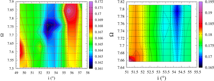
Figure 3. Contour plot of the inclination and surface potential (Ω–i) cross-section parameter hyperspace for both A (left) and W (right) subtypes; different shades of color represent the χ2, and our solution is located in the bluer region of the plot.
Download figure:
Standard image High-resolution image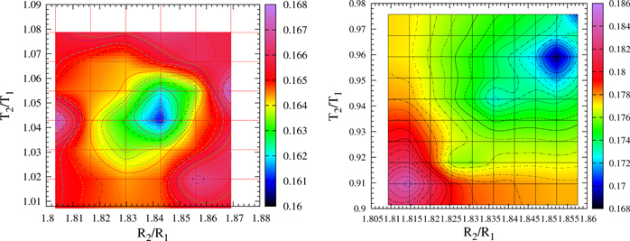
Figure 4. Contour plot of the effective temperature ratio and radius ratio of the components ( -
-  cross-section) for both A (left) and W (right) subtypes; different shades of color represent the χ2, and our solution is located in the bluer region of the plot.
Download figure:
Standard image High-resolution imageThe addition of spots in the initial model was further tested using the F test (Numerical Recipes, Press et al. 1986) to examine if the variances of the two models (spotted – unspotted) are equal. The summary statistics indicates that for the case of Model 1, F = 1.3151 with a probability of 4.75 × 10⁻⁸, and for the Model 2, F test = 1.2610 with a probability of 3.7 × 10⁻⁶. Thus in both cases the probability of equal variances between spotted and unspotted models is low.
Finally, the three-dimensional models for both spotted solutions of A and W subtypes are shown in Figures 5(a) and (b), respectively (making use of the Binary Maker 3 program; Bradstreet & Steelman 2002).
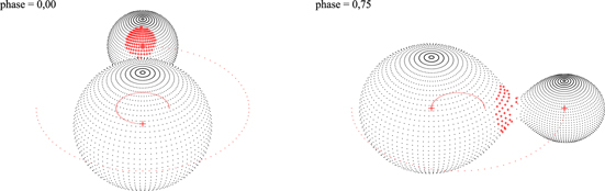
Figure 5. Geometrical representations of HI Dra Model 1 at phase 0.0 (left) and Model 2 at phase 0.75 (right).
Download figure:
Standard image High-resolution image5. DISCUSSION
In this study two spotted models are proposed for the overcontact system HI Dra that are investigated thoroughly through MC/heuristic scanning with parameter kicking in order to escape local minima and compute the parameters of the system with statistical and more realistic errors. According to our analysis, the new V, Rc, Ic CCD photometric data in combination with the spectroscopic information from the literature reveal that HI Dra can be described in two ways: an A subtype with a cool spot on the less massive component or a W subtype with a hot spot on the massive component. Although it is not easy to discriminate between the two (both models predict both the photometric and spectroscopic observations), according to the weighted sum of the squared residuals between the observed and synthetic LCs, the best model is described with the A subtype configuration, which also has the advantage of decreasing the extremely high temperature difference of the components ( = 0.830 ± 0.006 for the initial W subtype model). The combination of our LC solutions with RV information allows us to compute the absolute parameters of the system. After acquiring the temperature ratio
  and ratio of relative radii, we derived each component's effective temperature using Equation (3) from Zwitter et al. (2003) after disentangling the effective temperatures based on their effective temperature ratio derived from the model and the assumed F1V system's spectral classification. The resulting parameters of HI Dra are given in the lower part of Table 3 with their statistical/propagated errors described in the previous section.
In order to determine which model is more physically probable, we overplotted the modeled components in the mass–luminosity plane (Figure 6) together with other well-studied overcontact binaries. The data are taken from the compilations of Yakut & Eggleton (2005), Li et al. (2008), and Christopoulou et al. (2012). As can be seen in the figure, the location of the binary components favors the general pattern of A subtype W UMa systems. The primary star lies in the main-sequence band, while the secondary (less massive) is oversized and oveluminous for its mass. Actually, the radius of the secondary is 1.08 ± 0.02  , nearly twice that of a main-sequence star with M = 0.43 ± 0.02
  , and follows the general radius difference of other A-type W UMa binaries found by Yildiz & Doğan (2013). In combination with the temperature difference between the components, there has probably been a past epoch of mass transfer. Although the primary component, with a mass of 1.72 ± 0.08
  and a radius of 1.98 ± 0.03
  , lies in the main-sequence band, the zero-age radius inferred for a star of that mass (approximately 1.55
  ) suggests that the system is somewhat evolved, consistent with the A-type classification. The mass–radius diagram for the primaries of 51 A and 49 W subtype W UMa binaries of Yildiz & Doğan (2013, their Figure 1(b)) can be used as a consistency check of the above. Thus our light and velocity solutions indicate that HI Dra is a low inclination eclipsing A-type overcontact binary with a fill-out factor of about 24% and a temperature difference of 330 K between the components. The binary model with a single cool spot on the less massive secondary component fits all available LCs quite well.

Figure 6. Location of the components of HI Dra on logM–logL for both A and W subtype W UMa type eclipsing binary systems. Triangles and circles denote the more massive components (primaries) and rotated triangles and squares denote the less massive components (secondaries) of A and W subtypes, respectively. Full symbols are used for the components of HI Dra and open symbols for the others. The sample of W UMa type systems in the logM–logL diagram is taken from a compilation of Yakut & Eggleton (2005) and Li et al. (2008), updated and enriched from Table 9 of Christopoulou et al. (2012). The lines plotted using the BSE code (Hurley et al. 2002) are for the solar metallicity, ZAMS (solid line), and TAMS (dotted line).
Download figure:
Standard image High-resolution image
Recently, Yildiz & Doğan (2013) developed a method for the computation of initial masses of contact binaries based on stellar modeling with mass loss from luminosity excess. Their main assumption is that the mass transfer starts near or after the TAMS phase of the initially massive component, which is the progenitor of the currently less massive component. They discovered that binary systems with an initial mass higher than 1.8 ± 0.1  become A subtype, while systems with initial masses lower than this become W subtype. By applying their method to HI Dra, we found that the initial mass of the currently less massive component (0.43 ± 0.02
  ) would be 2.25 ± 0.07
  , that is, HI Dra should have evolved to an A subtype as predicted by our best model. With an initial mass of the HI Dra currently massive component calculated as 1.11 ± 0.03
  , the calculated initial total mass of the system (3.36
  ) is in good agreement with the mean total initial mass for a typical A subtype of 3
  (Yildiz & Doğan 2013). Moreover, following the procedure described by Yıldız (2014), we estimated the current age (the summation of the durations of three phases: detached, semidetached, and contact) of the HI Dra binary system to be approximately 2.4 Gyr.
Unfortunately, the limited number of times of minima does not allow the detection of any orbital period variation that may imply mass transfer between the components. Consequently, more accurate and dedicated times of minima for an extended period of time are required in order to study the period variation of HI Dra. Finally, we note that while this paper was under review, Caliskan et al. (2014) independently submitted a new study of the HI Dra system, together with other overcontact systems. Although their derived absolute parameters are in good agreement with ours, we propose a more propable configuration (A subtype) derived from the above detailed analysis of the parameter hyperspace and the evolutionary status of the eclipsing binary system. Nevertheless, without additional observational constraints like Doppler tomography, it is not possible to determine the true configuration of the spots on the stellar surfaces.
Footnotes
- 1
- 2
- 3