


ABSTRACT
We present the second realization of the International Celestial Reference Frame (ICRF2) at radio wavelengths using nearly 30 years of Very Long Baseline Interferometry observations. ICRF2 contains precise positions of 3414 compact radio astronomical objects and has a positional noise floor of ∼40 μas and a directional stability of the frame axes of ∼10 μas. A set of 295 new "defining" sources was selected on the basis of positional stability and the lack of extensive intrinsic source structure. The positional stability of these 295 defining sources and their more uniform sky distribution eliminates the two greatest weaknesses of the first realization of the International Celestial Reference Frame (ICRF1). Alignment of ICRF2 with the International Celestial Reference System was made using 138 positionally stable sources common to both ICRF2 and ICRF1. The resulting ICRF2 was adopted by the International Astronomical Union as the new fundamental celestial reference frame, replacing ICRF1 as of 2010 January 1.
Export citation and abstract BibTeX RIS
1. INTRODUCTION
The first realization of the International Celestial Reference Frame (hereafter referred to as ICRF1) (Ma et al. 1998) was the realization of the International Celestial Reference System (ICRS) (Arias et al. 1995) at radio wavelengths. It was defined by the very long baseline interferometry (VLBI) positions of 212 "defining" compact radio sources. These positions were independent of the equator, equinox, ecliptic, and epoch, but were made consistent with the previous stellar and dynamical realizations within their respective errors. The ICRF1 was constructed using geodetic/astrometric VLBI data taken between 1979 August and 1995 July, and contained 608 sources. It was adopted by the International Astronomical Union (IAU) as the fundamental celestial reference frame, replacing the FK5 optical frame (Fricke et al. 1988) as of 1998 January 1. Two extensions, ICRF-Ext.1 and ICRF-Ext.2, adding 109 additional sources (Fey et al. 2004), were later made using several years of newer VLBI data including the first of a series of Very Long Baseline Array (VLBA)23 Calibrator Surveys (VCS) (Beasley et al. 2002). In both extensions, the coordinates of the defining sources were kept unchanged from ICRF1. Maintenance of the ICRS is the responsibility of the International Earth Rotation and Reference Systems Service (IERS) with the International VLBI Service for Geodesy and Astrometry (IVS) having operational responsibility for the VLBI realization.
ICRF1 had an estimated noise floor of 250 μas and an estimated axis stability of ∼20 μas. This represented roughly an order of magnitude improvement over the previous stellar celestial reference frame, the FK5. Even so, ICRF1 had its limitations and deficiencies. The distribution of defining sources was very non-uniform, with most being in the northern hemisphere. Additionally, several of the original defining sources have subsequently been found to be unstable (showing significant systematic position variations), e.g., see Feissel-Vernier (2003).
Significant developments and improvements in the technique of geodetic/astrometric VLBI have been made since the generation of ICRF1. The sensitivity and quality of geodetic/astrometric VLBI data obtained by the IVS have improved significantly due to the use of wider single channel bandwidths, wider spanned bandwidths, receiver noise improvements, and better observing strategies. The use of newer and more sensitive antennas and arrays, such as the ten station VLBA, has greatly improved the sensitivity and quality of the data as well. Dedicated observing programs, such as the VLBA Research and Development VLBI (RDV) sessions, the southern hemisphere celestial reference frame sessions, the weekly large network dedicated Earth Orientation Parameter (EOP) sessions, and the VCS sessions have greatly improved the quality and quantity of the available VLBI data. Better geophysical modeling and faster computers have also allowed for significant improvements in the data analysis.
The amount of available VLBI data has increased by about a factor of four over ICRF1. The number of sources has also increased substantially. The ICRF1 contained 608 sources and was later expanded to 717. There are currently over 1200 sources whose positions can be obtained from the geodetic/astrometric sessions, and the number of southern hemisphere sources with precise positions has increased dramatically. When we include the purely astrometric VCS sessions, positions for nearly 2200 additional sources can be added, for a total of 3414 sources. The additional data also allows us to filter out the most unstable sources for special handling, avoiding possible distortion of the frame that might otherwise occur. There is now also a large amount of imaging data (e.g., the USNO Radio Reference Frame Image Database24 and the Bordeaux VLBI Image Database25 ), mostly from analysis and imaging of the RDV sessions. Sources with extensive intrinsic structure, which can contribute to apparent source proper motion, can thus be identified and eliminated from use in defining the reference frame.
The improvements in technique, modeling and the significantly larger amount of available data discussed above suggest that a set of more positionally stable sources distributed more uniformly over the sky could be selected to more precisely define the frame axis for an improved realization of the ICRF. Consequently, in 2006 the IAU formed a working group to oversee generation, validation and utility of a second realization of the ICRF. An IERS/IVS Working Group was then formed to generate the second realization of the ICRF from VLBI observations of extragalactic radio sources, consistent with the current realizations of the ICRS (ICRF1), the International Terrestrial Reference Frame (ITRF) and EOP data products. These international working groups were formed with members from the USA, France, Germany, Italy, Russia, Ukraine, Australia, and China. This paper summarizes the work of the IERS/IVS Working Group in its effort to generate a second realization of the International Celestial Reference Frame, hereafter referred to as ICRF2. More detailed technical information on ICRF2 can be found in IERS Technical Note No. 35 (Fey et al. 2009).
2. THE DATA
VLBI observations for geodesy and astrometry have been conducted since about mid-1979. A summary of the usage of VLBI data for celestial reference frames can be found in Gontier et al. (1997). Group delay observations are made in a bandwidth synthesis mode at standard frequencies of 2.3 GHz (S band) and 8.4 GHz (X band). The combination of observations at both bands allows for a first order correction of the dispersive effects of the Earthʼs ionosphere. At most stations a phase-calibration signal is injected into the radio receiver at both bands to remove instrumental dispersion and time variations in instrumental delay and meteorological information is logged during observations for use in tropospheric modeling. Observing sessions are typically of 24 hr duration as this period of time is required to recover (separate) parameters for nutation and polar motion and to average out remaining unmodeled geophysical effects.
The astrometric results presented here come from nearly 30 years of accumulated geodetic/astrometric VLBI observations. The earliest observations used are from 1979 August and the latest are from 2009 March and were obtained from many observing programs too numerous to list. Since 1999 these geodetic/astrometric observing programs have been coordinated by the IVS.
With few exceptions, the entire available VLBI data set was used, pooled cooperatively from all the various observing programs. Besides providing the potential for extracting the maximum information, the use of the entire data set includes the widest variation that the network geometry and station size can impose upon the realized ICRF2. The positions and stated uncertainties should then realistically represent how confidently the positions can be used in the future with arbitrary VLBI measurements. The VLBI data for this work were edited following the usual procedures of each contributing program. In the context used here, one observation represents one group delay measurement.
We briefly describe the three major sources of data used in this paper.
2.1. Geodetic/Astrometric VLBI
The geodetic/astrometric VLBI data set utilized for the construction of ICRF2 was obtained using a rich variety of stations and networks. The VLBI arrays used consisted of fixed and mobile antennas in configurations ranging from as few as two antennas (a single baseline) to as many as 20 antennas. Antenna sizes ranged from 3 up to 100 m. Unfortunately, the geographical distribution of the fixed VLBI antennas is very uneven. Out of approximately 53 antennas used over the past 30 years, only about ten were located in the southern hemisphere. Currently, there are about 34 fixed antennas that regularly or occasionally participate in geodetic/astrometric sessions, but only seven of those are in the southern hemisphere. This uneven geographical distribution directly affects the quality and quantity of data available in the southern hemisphere. The number of observations drops off rapidly for sources south of around −30° decl. In recent years, the IVS through its dedicated southern hemisphere observing program, has made great efforts to observe new sources in the southern hemisphere and to increase the number of observations of existing sources, with only moderate success due to limited resources.
2.2. VLBA RDV
The VLBA is an astronomical array of ten 25 m antennas. The VLBA antennas are some of the most sensitive and phase stable systems available. Details of their geodetic/astrometric use are given by Petrov et al. (2009). Use of the VLBA antenna at Pie Town, NM began in 1988 followed by the Los Alamos, NM antenna in 1991. Use of all ten VLBA antennas, and correlation on the VLBA correlator began in 1994. In a 2004 study, Gordon (2004) found that the regular VLBA (non-VCS) observations accounted for some 30% of the available geodetic/astrometric VLBI data and its usage improved the repeatability of the antenna positions at non-VLBA sites by typically 10%–40% and reduced the average source position formal uncertainties by ∼62% in R.A. and ∼54% in decl. for sources north of −30° decl. Currently, VLBA data comprises ∼28% of all the data used in this paper.
2.3. VLBA VCS
The VCS were a series of six multi-session S/X-band astrometric campaigns designed to image and find precise positions of as many new compact radio sources as possible for use by the radio astronomical community as VLBA phase reference calibrators. The first of these campaigns, VCS-1, was observed during 1994–1997. The resulting ten 24 hr sessions are described and analyzed by Beasley et al. (2002). An eleventh VCS-1 session, initially considered a failure, was later recovered and re-analyzed successfully. Five follow up VCS campaigns were made between 2002 and 2007 by Fomalont et al. (2003), Petrov et al. (2005, 2006, 2008) and Kovalev et al. (2007). These observing campaigns added another thirteen 24 hr sessions for a total of 24 VCS sessions. The observing mode was modified from that of regular geodetic/astrometric sessions. The VCS sessions concentrated on making short duration observations of many new sources as opposed to repeated observations of a smaller set of known sources. The sessions were not optimized for full sky coverage nor for atmospheric calibration, although the later sessions were better calibrated than the first sessions. The VCS sessions add nearly 2200 additional sources, with most of those observed in only one VCS session.
3. PREPARATION FOR ANALYSIS
3.1. Selection of the Analysis Software
The Working Group had access to several VLBI software analysis systems including: CALC/Solve (Ma et al. 1986); OCCAM (Titov et al. 2004); SteelBreeze developed at the Main Astronomical Observatory of the National Academy of Sciences of Ukraine (MAO) and Quasar developed at the Institute of Applied Astronomy of the Russian Academy of Sciences (IAA). See Fey et al. (2009) for additional information on these VLBI analysis packages.
For ICRF2, two overarching questions needed to be answered: (1) would the source positions come from a single solution generated with a single software analysis package or would they be the result of a combination catalog (i.e., the positions would be the averaged values from those generated with different analysis packages appropriately weighted by the formal uncertainties); and (2) if a single solution, which software analysis package would best suit the requirements for ICRF2.
The Working Group examined the available software analysis systems and used them to study, characterize and analyze the available VLBI data. Preliminary analysis of the data included the generation and study of source position time series to identify stable and unstable sources, the generation and inter-comparison of preliminary source position catalogs generated independently using the different analysis systems and analysis options, and the creation and study of a combination catalog based on the preliminary catalogs. Detailed results of these studies can be found in Fey et al. (2009). In the end, the Working Group decided to use a single catalog rather than a combination catalog for several reasons. The position catalogs from the separate software analysis packages going into the combination catalog differed slightly due to small differences in the underlying geophysical modeling, in editing criteria of the raw data, and/or in the amount of data used and its overlap. Additionally, a combination catalog with existing software loses certain information such as the full covariance matrix and the links to EOP products and the ITRF. See Sokolova & Malkin (2007) for a more thorough discussion on comparison and combination of radio source position catalogs.
The Working Group decided that the solution used to estimate positions for ICRF2 would be made at the National Aeronautics and Space Administration (NASA) Goddard Space Flight Center (GSFC) using the CALC/Solve package, primarily as a matter of convenience and the fact that the GSFC system had access to the most complete set of VLBI data. Similar results could have been obtained with the other analysis systems but with greater effort. Although the final ICRF2 catalog is based on a single solution done at the GSFC, the generation of ICRF2 could not have been realized as accurately and with as much understanding of the limiting errors and noise levels without access to the OCCAM, SteelBreeze and Quasar VLBI software analysis packages. Detailed comparison of the analysis software, described in more detail in Fey et al. (2009) gives confidence in the correctness of the mechanical implementation of the VLBI modeling.
3.2. Selection and Treatment of Special Handling Sources
Variable intrinsic source structure can contribute to apparent source proper motion, e.g., due to changes of the position on the sky of the brightness peak of a core-jet source. In this section we attempt to identify the worst such sources so that their effect on the reference frame can be minimized.
A series of global solutions was made. In each solution the positions of all sources except for a small test set were estimated as time-invariant "global" parameters. The positions of the test sources were treated as "arc" parameters with a position estimated for each day the source was observed. Each source was treated as a test source in some solution. The complete set of source positions as functions of time was then analyzed to determine which sources had statistically significant variations in their positions.
Statistics of these position time series in R.A. and decl. were calculated and examined, such as weighted root mean square (wrms) variations about the mean, χ2 per-degree of freedom and smoothed 2 year linear slopes. A total of 39 sources showing the largest position variations were selected in this manner for special handling. These sources show significant position variation in either R.A. and/or decl. and were observed historically in many sessions. Some of these are strong sources that have not been observed very often in recent years because of known adverse source structure effects on geodetic solutions (such as 3C84, 3C273B, 3C279, 3C345, and 3C454.3). A few are sources that are not very well observed overall, but still show convincing systematic position variations. Estimating the positions of these sources as global parameters would introduce significant systematic position errors and yield grossly underestimated position uncertainties that could possibly distort the overall reference frame. Therefore the positions of these sources were treated as arc parameters in the final global solution.
The 39 special handling sources are: 0014+813, 0106+013, 0202+149, 0208−512, 0212+735, 0235+164, 0238−084 (NGC 1052), 0316+413 (3C84), 0430+052 (3C120), 0438−436, 0451−282, 0528+134, 0607−157, 0637−752, 0711+356, 0738+313, 0919−260, 0923+392 (4C39.25), 0953+254 (OK 290), 1021−006, 1044+719, 1226+023 (3C273B), 1253−055 (3C279), 1308+326, 1404+286 (OQ 208), 1448+762, 1458+718 (3C309.1), 1611+343, 1610−771, 1641+399 (3C345), 1739+522, 2121+053, 2128−123, 2134+004 (2134+00), 2145+067, 2201+315, 2234+282, 2243−123, and 2251+158 (3C454.3). Seven of these sources (marked in italics) were original ICRF1 defining sources.
Note that it should not be assumed that there are only 39 unstable sources among the available sources. The vast majority of the sources have not been observed with the frequency necessary to detect the type of small systematic position variations seen in some of these sources. Many other sources showed smaller position variations that could, with more observation, show larger variability that would exclude them in the future. In such cases, it would seem that more data is not necessarily a good thing. We have attempted only to identify the worst such sources with the available data to minimize their effect on the reference frame.
Finally, there are a few sources excluded from the final global solution for various other reasons. Included in this category are three known gravitational lens sources and six known radio stars. The gravitational lens sources present analysis problems in assigning a single position and the radio stars exhibit real proper motion and are thus unsuitable for the purposes of a reference catalog. Also excluded from the final global solution were 795 sources with insufficient data for position determination. These sources were observed unsuccessfully for unknown reasons but are included in the VLBI data set for historical reasons and can be deselected when the analysis is done. Most of these sources were in the VCS sessions and are assumed to be either too weak or too spatially extended for reliable detection.
4. THE CALC/SOLVE ANALYSIS SOFTWARE
The GSFC analysis system consists of the astrometric and geodetic VLBI reduction software CALC and Solve. The data analysis methods using the GSFC system are covered in detail in Ma et al. (1986) and will be described only briefly here. CALC calculates the observation equations including most partial derivatives and contains most of the physical models of the reduction process, generally following, e.g., the IERS Conventions (2003) (McCarthy & Petit 2004). Solve uses the output of CALC, along with some additional modeling, to perform a least-squares solution to estimate parameters such as source or station positions, EOPs. Solve can be run in interactive mode for single VLBI experiments or in a non-interactive mode so that data from different experiments can be combined, allowing some parameters (e.g., source positions) to be estimated from a combination of many data sets.
To obtain a least-squares solution, the individual data sets are combined sequentially using "arc"-parameter elimination (Ma et al. 1990). All solutions give weighted least-squares estimates for parameters. Time-invariant or "global" parameters, i.e., parameters dependent on all data sets, are carried from step to step resulting in a single estimate derived from the combined data of all experiments in the solution. Depending on the problem at hand, these global parameters may include station positions, station velocities, source positions, source velocities (proper motions), nutation series coefficients, the precession constant, Love numbers for some solid Earth tides, and the relativistic gamma factor. Local or "arc" parameters depend only on the data from an individual experiment and are estimated separately for each epoch of observation. Arc parameters may include those for the station clocks and atmospheres, the Earthʼs orientation, and nutation offsets in obliquity and longitude. Station positions and source positions can also be arc parameters if the solution is to follow changes over time.
The astrometric positions given in this paper result from a particular choice of analysis configuration as described in following sections.
5. TYPE OF SOLUTION: TERRESTRIAL REFERENCE FRAME (TRF) VERSUS BASELINE
One of the requirements for ICRF2 was that it should be consistent with the current realization of the ITRF and EOP data products. In practice, this means that it should be consistent with VTRF2008 (Böckmann et al. 2010a), the VLBI determined input to the ITRF (ITRF2008).
There are two basic ways of treating the VLBI antenna positions and velocities in a Solve global solution. In a "baseline" type solution, site positions are treated as arc parameters, and separate positions are obtained for each session in which an antenna participated. In a baseline solution, no-net-translation constraints are applied to the estimation of site coordinates for each session individually and EOP are normally fixed to an a priori series. In a "TRF" type solution, positions and velocities are solved globally from the entire data set resulting in a single position and velocity estimate for each antenna at a specified epoch. In a TRF solution, no-net-rotation and no-net-translation constraints are applied globally to the positions and velocities of a set of core antennas, deemed to be stable and without discontinuities, to align the set of global antenna positions and velocities with an a priori reference frame. Antennas that show position discontinuities, e.g., due to earthquakes or mechanical movement of the antenna, must be modeled separately to account for the discontinuous antenna position. EOP are estimated for each session with the exception of single baseline sessions.
The solutions used for ICRF1 and its extensions were of the baseline type. In order to be consistent with the current realization of the ITRF and EOP products and to facilitate comparison, the final ICRF2 solution was chosen to be of the TRF type. Further discussion on how this choice affects source position estimation can be found in Section 7.1.
6. CONFIGURATION OF THE ICRF2 SOLUTION
The final analysis for ICRF2 was made at the GSFC using the CALC/Solve VLBI analysis package. The configuration of the ICRF2 solution was developed as a balance between competing goals: the most data and the least systematic error; the best models and available options; the largest number of useful estimated parameters and computer speed, etc.
Only observations above 5° elevation were included in the solution due to inadequacies in modeling the troposphere at lower elevations. The troposphere was modeled using the Vienna Mapping Function (VMF1) (Böhm et al. 2006). Atmospheric pressure loading corrections were applied according to Petrov & Boy (2004). The antenna thermal deformation model of Nothnagel (2008) was also applied.
The weighting of the data followed the usual GSFC procedure. For each experiment session, an added noise value is calculated for each baseline so that the reduced  is close to unity when the re-weighted noise is added quadratically to the measurement uncertainty determined from the correlation, fringe-fitting, and ionosphere calibration process. First order ionosphere corrections were made using a combination of the S band and X band group delay observables.
The a priori models for geophysical effects and precession/nutation generally followed the IERS Conventions (2003) (McCarthy & Petit 2004). Specifically, corrections for solid Earth tides, the pole tide, ocean loading, and high frequency EOP variations were made using those prescribed by IERS Conventions (2003).
As mentioned previously, parameters were estimated using arc-parameter elimination (Ma et al. 1990), which is an incremental least-squares method that can accommodate large numbers of parameters if they are associated only with particular data intervals or "arcs." For each observing session, the adjusted arc parameters included: quadratic clock polynomials for the slowly varying gross clock behavior; piecewise linear continuous functions at 60 minute intervals for short-term clock behavior; station wet troposphere zenith delays as piecewise linear continuous functions at 20 minute intervals; atmosphere gradient residuals from an a priori gradient model (MacMillan & Ma 1997) in the N–S and E–W directions estimated at six hour intervals; UT1 and polar motion offsets and rates estimated at the midpoint of each session; nutation offsets estimated at the midpoint of each session; and necessary nuisance parameters such as clock jumps and baseline clock offsets (i.e., separate bias parameters for each VLBI baseline to accommodate small, constant, baseline-dependent instrumental and correlator errors). Source positions for the set of 39 "special handling" sources whose time series exhibited clear systematic position variations (see Section 3.2) were also estimated as arc parameters.
The remaining parameters were adjusted as invariant quantities from the entire data set. These "global" parameters included: source positions for all sources with three or more successful group delay observations; station positions; station velocities; and antenna axis offsets.
The final global solution (designated ICRF2gsfc to indicate that this is an intermediate result) used a total of 4540 VLBI sessions with a total of 6,495,553 group delay measurements from observations obtained during sessions ranging from 1979 August 3 to 2009 March 16. The overall wrms post-fit delay residual was 21.85 ps and the reduced  was 0.89. "Global" positions were obtained for 3375 sources, and "arc" positions (time series positions) were obtained for the 39 special handling sources. The positions reported in this paper for these thirty-nine sources are the weighted means of their time series positions and the reported uncertainties are the wrms positions about the weighted means. Thus, positions and uncertainties for a total of 3414 sources are reported.
7. DETERMINATION OF REALISTIC ERRORS
The formal uncertainties of source position estimates based on observation noise tend to improve by a factor of 1/ where N is the number of observations. Consequently, for sources that have a very large number of observations, the formal uncertainties are generally unrealistically small and tend not to account for systematic errors.
To obtain a more realistic measure of the uncertainty, we have considered three effects: (1) modeling and data errors, (2) analysis noise, and (3) statistical consistency (validity) of the formal uncertainties.
7.1. Modeling Errors
We performed CALC/Solve test solutions to determine the sensitivity of the source position estimation to different model choices, solution strategy and choice of included data.
The model choices investigated were: (1) application of atmospheric pressure loading, (2) the VMF1 (Böhm et al. 2006) versus the NMF (Niell Mapping Function) (Niell 1996) troposphere mapping functions, (3) application of antenna thermal deformation (Nothnagel 2008), and (4) estimation of troposphere gradients with relatively tight constraints using an a priori gradient model versus estimation of total gradients with very loose constraints. Results of these comparisons are listed in Table 1 as weighted mean and wrms differences in source position estimations between the various solutions. Also listed are the overall rotation angles between the positions from the various pairs of solutions.
Table 1. Summary of Data and Model Comparisons
| Data/Model Comparison |
 αcosδ
αcosδ
|

|
Rotation Angles | ||||
|---|---|---|---|---|---|---|---|
| mean | wrms | mean | wrms | X | Y | Z | |
| (μas) | (μas) | (μas) | (μas) | (μas) | (μas) | (μas) | |
| Pressure Loading: On versus Off | 0 | 2 | 0 | 3 | 2 | 1 | 0 |
| VMF1 versus NMF | −1 | 3 | −3 | 5 | −1 | 2 | −1 |
| Thermal Deformation: On versus Off | 0 | 0 | 0 | 1 | 0 | 0 | 0 |
| Gradients: a priori versus no a priori | 0 | 7 | 6 | 12 | 8 | 5 | 3 |
| TRF versus Baseline | −1 | 10 | 0 | 12 | 2 | 2 | 2 |
| Start Time: 1990 versus All | 1 | 8 | 1 | 11 | 0 | 2 | 1 |
| Start Time: 1993 versus All | 0 | 14 | 0 | 18 | −1 | 5 | 4 |
Download table as: ASCIITypeset image
To assess the effect of solution type on source position estimates, we compared results from a baseline type solution with those from a TRF type solution. As discussed in Section 5, the ICRF2gsfc solution was chosen to be of the TRF type in which station positions and velocities are solved globally from the entire data set resulting in a single position and velocity estimate for each antenna at a specified epoch as opposed to a baseline type solution in which site positions are treated as arc parameters and separate positions are obtained for each session in which an antenna participated. This comparison essentially quantifies the effect of daily station motion on global source position estimates. These results are also listed in Table 1.
Finally, test solutions were made including data starting from 1990 or 1993 compared with the entire data set spanning 1979–2009. The chronologically earlier VLBI data is known to be considerably noisier than later data. This is due to many improvements over the past 30 years, such as increased individual channel bandwidths, increased spanned bandwidths, improved electronics, new and more sensitive antennas, larger networks, improved scheduling methods, and other factors. These results are also listed in Table 1.
The results presented in Table 1 show that uncertainties due to our choice of modeling options, the solution type and/or choice of included data are all well within the estimates of the noise floor and axis stability discussed in Sections 7.3 and 11.3, respectively.
7.2. Analysis Noise
Analysis noise refers to the cumulative effects of data editing and/or modeling errors in the resulting source position estimates from a global VLBI solution. One way of estimating the magnitude of this error is to compare solutions performed by different VLBI analysis centers using different software and/or modeling, where each center starts with the same observational data.
The wrms difference between source position estimates, si, from two global solutions after removing biases is
where  are the estimated variances of the source positions and the position estimates from the two solutions are assumed to be uncorrelated. If we assume the two solutions have the same noise then we can get an estimate of the noise of each solution,
  .
.
Table 2 lists the wrms differences (scaled by a factor of 1/ ) between the ICRF2gsfc solution and several solutions from other analysis centers, namely USNO, IAA and MAO. VCS sources from these solutions were not included in the comparisons. The listed scale factors are the
  of the differences scaled by the formal uncertainties of the solutions. These differences give a measure of the analysis noise inherent in the solutions. The GSFC/USNO differences are generally the smallest since both solutions used the CALC/Solve analysis software. The IAA and MAO differences tend to be larger presumably because these solutions used different analysis software, i.e., QUASAR for IAA and SteelBreeze for MAO.
Table 2. Solution Difference Statistics
| Solution | R.A. | Decl. | Number of Sources | ||
|---|---|---|---|---|---|
| wrms | Scale Factor | wrms | Scale Factor | ||
| (μas) | (μas) | ||||
| GSFC-USNO | 39 | 0.91 | 32 | 1.17 | 1136 |
| GSFC-IAA | 55 | 1.14 | 38 | 1.06 | 1051 |
| GSFC-MAO | 66 | 1.37 | 48 | 1.31 | 1031 |
| Decimation | 67 | 1.60 | 52 | 1.54 | 730 |
Download table as: ASCIITypeset image
As an additional estimate of realistic source position noise levels, we did a decimation test in which all included sessions were ordered chronologically and divided into two sets selected by even or odd session. Results of this test are also listed in Table 2 but discussed in Section 7.3.
7.3. Statistical Validity of the Formal Uncertainities
If all errors were Gaussian then the uncertainty of position estimates should fall off as 1/ where N is the number of observations. To determine a realistic level of source position errors, we ran a decimation test in which all VLBI experiment sessions were ordered temporally and divided into two independent data sets selected by even or odd session. This was done for each well-defined session type, where the session type refers to a series of experiments with the same core network of observing stations. This should help ensure that the two full sets of sessions were equivalent in terms of networks and sources observed. The remaining group of sessions not in an obvious category were similarly divided. Global solutions were performed with each set of sessions. Source position estimates from the two solutions are independent and the solution position differences yield estimates of the noise of each solution as well as how much the formal uncertainties should be scaled. The differences in source position estimates from the two decimation solutions were scaled by their formal errors and then the standard deviation of the scaled differences was computed. The resulting scaling factors (standard deviations) of 1.6 and 1.5 for R.A. and decl., respectively, are listed in Table 2 and can be compared to the scale factors arising from differencing solutions from different analysis centers, also given in Table 2.
To obtain a better estimate of the systematic noise floor, the sources were ordered by the average number of experiment sessions in which a source was observed in the two decimation solution. The differences in position were analyzed for a running window of 50 sources in this ordered sequence of sources. We computed the wrms difference of positions from the two solutions for each 50 source subset of all the sources common to both decimation solutions. Figure 1 shows the dependence of the wrms difference (scaled by 1/ ) as a function of the minimum number of sessions in each subset. This is compared to the median formal uncertainty in the subset. The wrms differences are larger and fall off less steeply than the median formal errors, which fall off as 1/
 . The observed minimum error of 25 μas for decl. and 15 μas for R.A. is reached for sources that have been observed in more than 200 sessions. If one applies an overall scaling factor of 1.5 based on all source position differences, one still needs to add additional noise to account for residual scaling errors that are as large as 1.5 for sources observed in less than 75 sessions. At the expense of overly conservative uncertainties for the most well observed sources, we chose a noise floor of 40 μas, which is the noise level in Figure 1 for both R.A. and decl. for sources observed in at least 100 sessions.

Figure 1. wrms noise (solid circles) for subsets of 50 sources in each decimation solution as a function of the minimum number of sessions in which a source was observed. The median formal uncertainty (red triangles) in each subset is shown for comparison. These values were derived from differences between positions in the two decimation solutions discussed in Section 7.3.
Download figure:
Standard image High-resolution imageConsequently, the formal errors of the ICRF2gsfc catalog were inflated following the formula:


where the subscript zero indicates the formal errors. If we inflate the formal errors in this way, the average residual scaling factors are 0.95 for decl. and 0.88 for R.A.
8. CONSISTENCY WITH THE ITRF AND EOP PRODUCTS
The ICRF2gsfc solution represents the state-of-the-art astrometric position catalog at the time the solution was made. There are no other comparable catalogs that can be used to assess its own astrometric quality. However, as described in Section 6, the ICRF2gsfc solution results from an analysis in which radio source positions, VLBI antenna positions, antenna velocities and EOP products are all simultaneously estimated. As such, these parameters are consequently linked in a consistent and verifiable way. Thus, an external validation of the source position results can be carried out through an indirect quality assessment applied to the EOP and the TRF results alone.
8.1. Earth Orientation Parameters
The International GNSS Service (IGS), through observation and analysis of the Global Positioning System (GPS) satellites, provides a suitable external data set with the same or better quality for external validation of VLBI EOP products, but only for polar motion cf., Böckmann et al. (2010b). The other components of EOP, UT1-UTC and offsets in nutation angles, are the almost exclusive domain of VLBI and as such, for these components, no suitable external, i.e., non-VLBI, comparison is available.
We compared polar motion X and Y between the IGS EOP series and ICRF2gsfc together with those from five other VLBI global solutions contributed from the various VLBI analysis groups including BKG, USNO, MAO, IAA and the Observatoire de Paris (OPA). After subtracting an overall bias and rate between the IGS and VLBI series, the six VLBI solutions considered exhibit wrms agreement with the IGS series at the roughly 100 μas level in both the X and Y components. Noticeable systematic variations evident in the Y component from all the VLBI series have been identified with changes in the VLBI network arrays (Artz et al. 2008), but in general, the scatter between the different VLBI solution results and the systematic network effects are at the same level indicating that the wrms values are representative of the overall agreement between the IGS and VLBI polar motion values.
An evaluation of the other three components of the standard Earth orientation representation, UT1-UTC and nutation in dX and dY, can only be carried out by inter-comparison of the results of the six VLBI solutions mentioned in the previous paragraph. This is a valid approach here since the six VLBI EOP time series were generated using the three different and independent software packages CALC/Solve (BKG, GSFC, OPA, USNO), SteelBreeze (MAO) and Quasar (IAA). The IERS EOP 05 C0426 (hereafter IERS C04) series was used as a standard reference to subtract a common signal from the six VLBI series. Note that this comparison does not represent a qualitative analysis of the differences between the VLBI series and IERS C04 in an absolute sense since the IERS C04 series is mainly derived from VLBI results but does represent the level of relative agreement.
Examination of the differences between the six VLBI series and IERS C04 show that there are no systematic differences in nutation angles between the four CALC/Solve solutions and the SteelBreeze solution. However, a very obvious systematic effect with an irregular period is present in the IAA time series. This effect was traced to errors in the relativistic model used in the submitted IAA EOP series. Since the MAO and IAA time series do not show strong correlations but the MAO series follows the four Calc/Solve solutions, albeit with some excess noise, it can be concluded that the inter-comparisons provide a reliable relative indication of the quality of each VLBI input series. The wrms agreement between the MAO nutation angle series and the IERS C04 series agrees at the ≈100 μas level in both nutation angles whereas the CALC/Solve solutions range in agreement at the 60–95 μas level. Since these time series all agree with the reference series at a similar level, the absolute accuracy of the nutation estimates should not be worse than by about a factor of  , thus indicating that the nutation angle accuracy is at the same level as that of polar motion.
A comparison of the six VLBI series for UT1-UTC shows that the reference series IERS C04 exhibits a long term drift after about epoch 2002.5. Nevertheless, the VLBI solutions all agree with each other at the few μs level. The wrms differences in UT1-UTC with respect to the reference series is at the level of about 9 μs which corresponds to 135 μas. This number is driven by the systematic effect in the differences and does not characterize the agreement of the six series as such. The agreement between the six VLBI series is rather at the 4–5 μs level corresponding to 100 μas which is the same level of agreement as the polar motion results and can, therefore, be considered as the upper limit also of this component of Earth rotation.
From the comparisons of the EOP results, it can be concluded that the six VLBI solutions agree with each other at the level of better than 100 μas excluding known systematic effects. The polar motion results of the VLBI series agree with the IGS GPS results at the ≈100 μas level and considering that the other EOP components do not exhibit any obvious systematic effects, it can be concluded that their accuracy is at the same level. Consequently, an upper bound of 110 μas or 3.3 mm at the Earthʼs surface can thus be inferred for the overall accuracy of each observing session contributing to the VLBI determination of ICRF2.
8.2. Terrestrial Reference Frame
A second option for external validation of the ICRF2gsfc solution is to investigate the accuracy of the station positions and velocities in terms of the quality of the TRF that they represent. As discussed in Section 6, station positions and velocities are estimated in the same solution as the source positions.
We compared the TRF from the ICRF2gsfc solution with VTRF2008 (Böckmann et al. 2010a), the VLBI determined input to ITRF2008. Ideally, a comparison should be made to ITRF2008, but unfortunately ITRF2008 had not been released at the time this work was done. VTRF2008 is a combination product with input from several IVS Analysis Centers and should provide a very reliable reference due to the stabilizing effect of the combination. Six of the seven input solutions used the CALC/Solve analysis software and one solution was generated using the OCCAM analysis software. Although it would be better to have more solutions from different independent software packages, the agreement of all the input solutions in general and the agreement of the TRF between the independent software packages of CALC/Solve and OCCAM in particular, should preclude any serious deficiencies in the combined TRF.
In order to facilitate comparison, a 14-parameter Helmert transformation between the ICRF2gsfc solution and the VTRF2008 were calculated. In the context of ICRF2, the rotations and their time evolution are of particular importance. The TRF from the ICRF2gsfc solution is rotated with respect to VTRF2008 but not by more than ∼40 μas. The rotation rates are at the level of a few μas year−1 with formal errors at about the same level. The scale difference and its rate with respect to VTRF2008 is not significant.
The quality of the coordinates and velocities of individual VLBI antenna sites can best be discussed by looking at the residuals of the antenna positions at epoch and their velocities. Antenna positions at sites actively observing at the reference epoch (J2000.0) generally show differences with respect to VTRF2008 below about 5 mm in their horizontal topocentric positions with matching discrepancies in the station velocity components. Notable exceptions are SYOWA and OHIGGINS, two VLBI stations located in Antarctica, the TIGOCONC station located in Chile and the NYALES20 station located in Norway, with residuals in the horizontal components being slightly larger. However, the differences in the vertical components of these four sites fit very well to VTRF2008. Other stations with larger residuals are older radio telescopes which either no longer exist or are no longer in use and hence do not have current data.
On the basis of the Helmert parameters of the ICRF2gsfc solution with respect to VTRF2008 it can be stated that the orientation of the TRF axes from the ICRF2gsfc solution matches the orientation of the VTRF2008 within ∼40 μas and a few μas year−1, respectively. The residuals of horizontal and vertical components of the station coordinates as well as of the velocities confirm the overall accuracy of the ICRF2gsfc solution at the level of about 3.5 mm.
9. CHARACTERIZATION OF SOURCE STRUCTURE
There is now a large amount of intrinsic source structure information available, mostly from analysis and imaging of the VLBA RDV sessions. Sources with extensive intrinsic structure, which can contribute to apparent source proper motion, can thus be identified and eliminated from use in defining the reference frame. These data can also be used to identify the most compact, and presumably most suitable, astrometric sources.
In order to assess the astrometric quality of the sources, we used the "structure index" (SI) defined by Fey & Charlot (1997), modified so as to obtain a SI on a continuous scale. The SI indicates the expected magnitude of the effects of intrinsic source structure on VLBI group delay observations according to the median value of the structure delay corrections,  , calculated for all projected VLBI baselines that could be theoretically observed with Earth-based VLBI, using the algorithm devised by Charlot (1990). While Fey & Charlot (1997) separated the sources into four categories, with quantized values of the SI ranging from 1 to 4, we adopt a continuous scale for the present work and define a continuous structure index
  as follows:

where  is expressed in picoseconds (ps). Additionally, the values of
  are constrained to remain positive by setting
  when
when  .
.
There is close correspondence at the (discrete) boundaries between the continuous  values defined here and the values defined in Fey & Charlot (1997), i.e.,
  versus 2 for
  ps,
ps,  versus 3 for
  ps and
  versus 4 for
  ps. The recommendation of Fey & Charlot (1997) that sources with SI values of 3 or 4 should not be used for high-precision VLBI astrometry therefore remains mostly valid with this new definition of the SI.
Based on the above definition,  was calculated for 707 sources at multiple epochs between 1994 and 2008 using a total of 3052 X band images from the USNO Radio Reference Frame Image Database and the Bordeaux VLBI Image Database. The vast majority of the images of the sources north of about −40° decl. were obtained from RDV sessions or from earlier VLBA sessions (Fey et al. 1996; Fey & Charlot 1997, 2000). For the sources in the far south, the images are from dedicated southern-hemisphere VLBI sessions (Ojha et al. 2004, 2005). The number of images per source varied widely with almost half of the sources (331 sources) having been imaged at only a single epoch whereas the most often observed source (0727–115) was imaged at 32 different epochs. For the sources imaged at more than one epoch, an additional step was taken and the mean
  over all epochs was calculated. The time series of
  were also examined to check for outliers, possibly caused by images with low dynamic range or poor resolution, which may affect the mean values, and for variability over time, which is indicative of variable intrinsic structure. Mean
  values, together with the number of images on which the mean
  values are based, are listed in Table 1 of Fey et al. (2009) for 707 sources.
The distribution of the mean  values is shown in Figure 2. These values peak at
  , corresponding to a value of
  ps. Also marked in Figure 2 are the special handling sources discussed in Section 3.2 (with the exception of 0438–436 which does not have a SI available). Based on SI alone, it is found that 26 of the special handling sources have a
  value larger than 3.0, which is an indication of extended emission, making them unsuitable for precise astrometry. Six of the remaining sources, with
  values less than 3.0, show variable
  indicative of temporal structure changes suggesting that they may show positional instability. Overall, more than 80% of the special handling sources are thus found to be unsuitable for high precision astrometry when considering solely their intrinsic structure, in agreement with the findings in Section 3.2.
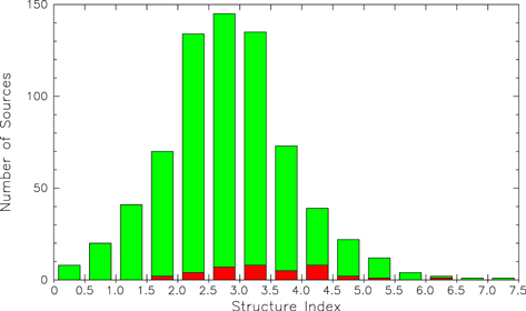
Figure 2. Distribution of the mean value of the continuous structure index ( ) for 707 sources with VLBI images available from the USNO Radio Reference Frame Image Database or the Bordeaux VLBI Image Database. The special handling sources discussed in Section 3.2 are color-coded in red.
Download figure:
Standard image High-resolution imageFinally, it should be noted that the  as calculated here represents only a snapshot of the intrinsic structure of these sources based on the imaging data available at the time this work was carried out and that these values may evolve with time.
10. SELECTION OF ICRF2 DEFINING SOURCES
Source positions estimated from the VLBI data analysis are of varying quality primarily due to different observing histories and astrometric suitability. In order to define a set of frame axes as accurately as possible, only the highest quality positions should be used for determining or "defining" the orientation of ICRF2. The remaining or "non-defining" sources, derived from the same solution as that of the defining sources, are included primarily to densify the frame. To be most useful in defining ICRF2, a source should ideally show no variation of position in the data set, have sufficient data to support the absence of variation and have minimal intrinsic source structure. In this section we attempt to establish an ordered list of defining sources based on their positional stability and on the cross-correlation between positional stability and source SI as defined in Section 9.
10.1. Positional Stability of Sources
Source ranking based on positional stability is derived using the position time series used to identify the 39 special handling sources in Section 3.2 and from the positions and uncertainties from the ICRF2gsfc catalog, after removing the 39 special handling sources. We start by keeping only the 593 sources whose positions were (1) estimated as global parameters in the ICRF2gsfc solution, (2) were observed in at least ten sessions, and (3) have an observational history of more than 2 years.
From the position time series, one can compute a positional stability index as

where  and
and  are the wrms position variations about the weighted mean position for R.A. and decl., respectively, and
  and
and  are the reduced
  of the fit to the mean positions.
From the ICRF2gsfc catalog, a combined formal error on the position estimate can be computed as

where  and
and  are the formal uncertainties in R.A. and decl., respectively, and
  is the correlation between estimates of α and δ.
If we naively define an overall positional stability index as  , we find that r is generally larger than d by about a factor of ten, further illustrating that the formal errors from the global solution are significantly underestimated. Thus a ranking based on p alone would be dominated by information primarily from the time series. Further, a ranking based on p alone rejects many of the southern hemisphere sources due to their poor observing histories. Consequently, we implement a method suggested by Fey et al. (2001) to select candidate defining sources which gives more equal weight to the wrms and formal uncertainties and which selects sources more uniformly distributed as a function of decl.
First, the 593 sources under consideration are divided into five approximately equal number bins based on decl. with boundaries at −31°, 0°, 18°, and 40°. Then, separately in each decl. band, sources are ranked on a normalized scale based on r alone. This normalized ranking is repeated but instead this time using the quantity d alone. Finally, the scaled r and d for each source are summed and re-normalized to a 0–100 scale. This final normalization constitutes the "quality" index P. The distribution of P is displayed in Figure 3.
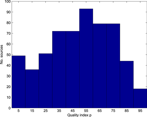
Figure 3. Distribution of the final quality index P.
Download figure:
Standard image High-resolution imageTests to determine the minimum number of sources required to define stable frame axes discussed in Fey et al. (2009) suggest that the minimum number of sources should be around 200 with an optimal value about 380, after which the stability is degraded. Thus we chose a value of quality index P ≥ 40 to give a list of 423 candidate defining sources.
10.2. Source Structure
The final list of defining sources results from the cross-correlation between the ranked list of sources described in Section 10.1, based on positional stability, and the ranked list of sources based on SI described in Section 9. Overall, the two criteria (positional stability and source SI) show good correlation with positional stability increasing as the SI decreases.
The initial list of 423 candidate defining sources was further narrowed by setting the threshold for the continuous SI to 3.0 (i.e., all sources with SI values larger than or equal to this threshold value were removed from the list). Thus, the final set of defining sources was reduced to 295 sources. Unfortunately, about 25% of these 295 sources, with most of them located in the southern hemisphere, had no SI available. These sources were kept on the basis of their positional stability alone.
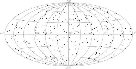
The distribution on the sky of the 295 ICRF2 defining sources is shown in Figure 4.
Figure 4. Distribution of the 295 ICRF2 "defining" sources on an Aitoff equal area projection of the celestial sphere. The dashed line represents the galactic equator.
Download figure:
Standard image High-resolution image
11. ALIGNMENT OF ICRF2 ONTO THE ICRS AND AXIS STABILITY
The VLBI analysis for the ICRF2gsfc catalog described in Section 6 provided accurate relative source positions and an overall orientation extremely close to that of the ICRS. However, the solution was not designed to obtain results directly on the ICRS. The final stage in the ICRF2 realization was the rigid rotation of the relative positions to the ICRS. The catalog was aligned to the ICRS by rotating it onto the frame defined by ICRF-Ext.2 using common sources.
11.1. Selection of Common Sources
Of the 295 sources selected as ICRF2 defining in Section 10, only 97 were also defining sources in ICRF1 (as realized by ICRF-Ext.2). Most of the overlap defining sources are in the northern hemisphere and hence are poorly distributed on the sky for reliable estimation of rotation angles between the two frames. To address this situation, an additional 41 of the 295 defining sources, mostly in the southern hemisphere, were selected resulting in 138 common objects for computation of rotation angles with the ICRF-Ext.2 catalog. The status of the additional 41 sources in ICRF-Ext.2 is: 24 candidate sources, 16 other, and 1 new.
11.2. Rotation
The ICRF2gsfc catalog (with inflated formal errors as described in Section 7) was compared to ICRF-Ext.2 using a 4-parameter transformation in which the coordinate differences are modeled by three rotation angles A1, A2 and A3, around the X, Y and Z axes of the celestial frame, respectively, and a parameter dz accounting for a global translation of the source coordinates in decl., e.g., see Feissel-Vernier et al. (2006):


The additional two deformation parameters used in the transformation formula for the alignment of ICRF1 (Ma et al. 1998) were found negligible and are not estimated here. Values of estimated parameters are listed in Table 3. The quantities  and
and  in Table 3 are the wrms residuals in
  and δ, respectively.
Table 3. Parameters to Transform ICRF2gsfc Onto ICRF-Ext.2
| A1 | A2 | A3 | dz |

|

|
|---|---|---|---|---|---|
| 23.3 ± 19.2 | −33.5 ± 19.5 | 7.8 ± 18.4 | 11.2 ± 16.6 | 9.2 | 12.4 |
Note. Unit is μas.
Download table as: ASCIITypeset image
Improvements in the models and procedures applied in the ICRF2gsfc catalog solution resulted in a frame with fewer deformations than ICRF-Ext.2, but with a slight mis-orientation. In the procedure applied to rotate the ICRF2gsfc catalog positions into the ICRS, care was taken not to transfer the deformations of ICRF-Ext.2 to ICRF2. Consequently the radio source coordinates of the ICRF2gsfc catalog were rotated onto the ICRS using only the three rotation angles A1, A2, and A3 listed in Table 3. The rotated ICRF2gsfc catalog constitutes the final ICRF2 catalog.
11.3. Axis Stability
The stability of the ICRF2 axes were tested by estimating the relative orientation between ICRF2 and ICRF-Ext.2, using Equations (6) and (7), on the basis of various sets and subsets of sources. The results of a sample of these comparisons is listed in Table 4. The scatter of the rotation parameters obtained in the different comparisons indicate that the axes are stable to within about 10 μas.
Table 4. Axis Stability Tests Between ICRF2 Defining and ICRF-Ext.2
| Subset of Sources | No. | A1 | A2 | A3 | dz | rαcosδ | rδ |
|---|---|---|---|---|---|---|---|
| Common | 245 | 5.2 ± 11.0 | −5.1 ± 10.5 | 14.0 ± 10.4 | 22.0 ± 10.0 | 5.3 | 7.4 |
| Link | 138 | 0.0 ± 19.2 | 0.0 ± 19.5 | 0.0 ± 18.4 | 11.1 ± 16.6 | 9.2 | 12.4 |
| Northern | 148 | 17.0 ± 10.7 | −1.2 ± 10.4 | 12.7 ± 10.7 | 26.1 ± 10.2 | 6.1 | 7.5 |
| Southern | 97 | −35.4 ± 28.0 | −18.6 ± 24.8 | 11.2 ± 22.3 | 19.9 ± 22.3 | 10.5 | 16.5 |
Note. Unit is μas.
Download table as: ASCIITypeset image
12. THE ICRF2 CATALOG
The final ICRF2 catalog is obtained from ICRF2gsfc after inflating the position formal errors as described in Section 7 and aligning the positions onto the ICRS as described in Section 11.2. It consists of positions of 3414 sources of which 2197 sources are observed only in the VCS sessions. Among the remaining 1217 sources, 295 have been designated as "defining" sources, i.e., the positions of these 295 sources define the axes of the ICRF2, as described in Section 10.
The coordinates of the 295 ICRF2 "defining" sources are listed in Table 5. Coordinates of the 922 ICRF2 non-VCS sources are listed in Table 6 and coordinates of the 2197 ICRF2 VCS-only sources are listed in Table 7. It should be noted that these positions are not epoch-dependent and hence no epoch is explicitly stated. However, the listed positions are consistent with epoch J2000.0.
Table 5. Coordinates of the 295 ICRF2 "Defining" Sources

|

|
Epoch of Observation | |||||||||
|---|---|---|---|---|---|---|---|---|---|---|---|
| Designationa | Sourceb | α | δ | (s) | ('') |

|
Mean | First | Last |

|

|
| ICRF J000435.6–473619 | 0002–478 | 00 04 35.65550384 | −47 36 19.6037899 | 0.00001359 | 0.0002139 | 0.383 | 52501.0 | 49330.5 | 54670.7 | 28 | 129 |
| ICRF J001031.0+105829 | 0007+106 | 00 10 31.00590186 | 10 58 29.5043827 | 0.00000491 | 0.0000930 | −0.187 | 53063.9 | 47288.7 | 54803.7 | 29 | 559 |
| ICRF J001101.2–261233 | 0008–264 | 00 11 01.24673846 | −26 12 33.3770171 | 0.00000660 | 0.0000936 | −0.183 | 52407.5 | 47686.1 | 54768.6 | 45 | 592 |
| ICRF J001331.1+405137 | 0010+405 | 00 13 31.13020334 | 40 51 37.1441040 | 0.00000482 | 0.0000683 | −0.139 | 51619.2 | 48434.7 | 54713.7 | 22 | 1083 |
| ICRF J001611.0–001512 | 0013–005 | 00 16 11.08855479 | 00 15 12.4453413 | 0.00000435 | 0.0001005 | −0.235 | 50403.0 | 47394.1 | 51492.8 | 67 | 716 |
| ICRF J001945.7+732730 | 0016+731 | 00 19 45.78641940 | 73 27 30.0174396 | 0.00000989 | 0.0000424 | −0.050 | 49249.8 | 44343.6 | 54865.7 | 458 | 25038 |
| ICRF J002232.4+060804 | 0019+058 | 00 22 32.44120914 | 06 08 04.2690807 | 0.00000439 | 0.0000956 | −0.237 | 52705.8 | 47394.1 | 54880.7 | 42 | 800 |
| ICRF J003824.8+413706 | 0035+413 | 00 38 24.84359231 | 41 37 06.0003032 | 0.00000499 | 0.0000613 | −0.035 | 52262.4 | 49422.9 | 54887.7 | 18 | 1024 |
| ICRF J005041.3–092905 | 0048–097 | 00 50 41.31738756 | −09 29 05.2102688 | 0.00000278 | 0.0000428 | −0.030 | 51323.1 | 44773.8 | 54816.7 | 1802 | 41482 |
| ICRF J005109.5–422633 | 0048-427 | 00 51 09.50182012 | −42 26 33.2932480 | 0.00000932 | 0.0001177 | 0.013 | 53857.8 | 52306.7 | 54907.7 | 31 | 315 |
Notes.
aICRF2 Designations, constructed from the source coordinates with the format ICRF JHHMMSS.s+DDMMSS or ICRF JHHMMSS.s-DDMMSS; they follow the recommendations of the IAU Task Group on Designations. bIERS Designations, previously constructed from B1950 coordinates; the complete format, including acronym and epoch in addition to the coordinates, is IERS BHHMM+DDd or IERS BHHMM-DDd.
Only a portion of this table is shown here to demonstrate its form and content. Machine-readable and Virtual Observatory (VOT) versions of the full table are available.
Download table as: Machine-readable (MRT)Virtual Observatory (VOT)Typeset image
Table 6. Coordinates of 922 ICRF2 (Non-VCS) Sources
| σα | σδ | Epoch of Observation | |||||||||
|---|---|---|---|---|---|---|---|---|---|---|---|
| Designationa | Sourceb | α | δ | (s) | ('') |

|
Mean | First | Last |

|

|
| ICRF J000108.6+191433 | 2358+189 | 00 01 08.62156690 | 19 14 33.8017390 | 0.00000490 | 0.0000984 | 0.080 | 53306.0 | 50085.5 | 54907.7 | 21 | 716 |
| ICRF J000211.9–215309 | 2359–221 | 00 02 11.98262436 | −21 53 09.8359742 | 0.00115400 | 0.0386714 | 0.971 | 54818.7 | 54818.7 | 54818.7 | 1 | 3 |
| ICRF J000435.7+201942 | 0002+200 | 00 04 35.75829931 | 20 19 42.3174919 | 0.00001434 | 0.0002426 | 0.079 | 52600.4 | 52409.7 | 52983.7 | 3 | 102 |
| ICRF J000557.1+382015 | 0003+380 | 00 05 57.17539168 | 38 20 15.1489409 | 0.00000488 | 0.0000621 | −0.083 | 52010.2 | 48720.9 | 54718.7 | 26 | 1518 |
| ICRF J000613.8–062335 | 0003–066 | 00 06 13.89288849 | −06 23 35.3353162 | 0.00000277 | 0.0000437 | −0.035 | 52342.2 | 47176.5 | 54889.8 | 1254 | 26713 |
| ICRF J000800.3–233918 | 0005–239 | 00 08 00.36965673 | −23 39 18.1511374 | 0.00002400 | 0.0007055 | −0.650 | 50918.1 | 50632.3 | 54643.7 | 3 | 95 |
| ICRF J001033.9+172418 | 0007+171 | 00 10 33.99063132 | 17 24 18.7613217 | 0.00000486 | 0.0000824 | −0.098 | 51780.9 | 47931.6 | 54844.7 | 40 | 1242 |
| ICRF J001052.5–415310 | 0008–421 | 00 10 52.51790008 | −41 53 10.7781702 | 0.00019412 | 0.0043581 | −0.068 | 50998.2 | 48162.4 | 52409.7 | 5 | 22 |
| ICRF J001135.2+082355 | 0009+081 | 00 11 35.26963063 | 08 23 55.5862723 | 0.00001305 | 0.0004120 | −0.455 | 52574.8 | 49914.7 | 53609.2 | 2 | 100 |
| ICRF J001708.4+813508 | 0014+813 | 00 17 08.47492105 | 81 35 08.1365288 | 0.00008598 | 0.0002624 | 0.000 | 50567.9 | 47023.3 | 54112.5 | 1185 | 61191 |
Notes.
aICRF2 Designations, constructed from the source coordinates with the format ICRF JHHMMSS.s+DDMMSS or ICRF JHHMMSS.s-DDMMSS; they follow the recommendations of the IAU Task Group on Designations. bIERS Designations, previously constructed from B1950 coordinates; the complete format, including acronym and epoch in addition to the coordinates, is IERS BHHMM+DDd or IERS BHHMM-DDd.
Only a portion of this table is shown here to demonstrate its form and content. Machine-readable and Virtual Observatory (VOT) versions of the full table are available.
Download table as: Machine-readable (MRT)Virtual Observatory (VOT)Typeset image
Table 7. Coordinates of 2197 ICRF2 (VCS-only) Sources
| σα | σδ | Epoch of Observation | |||||||||
|---|---|---|---|---|---|---|---|---|---|---|---|
| Designationa | Sourceb | α | δ | (s) | ('') |

|
Mean | First | Last |

|

|
| ICRF J000020.3–322101 | 2357–326 | 00 00 20.39994757 | −32 21 01.2335157 | 0.00003337 | 0.0009246 | −0.004 | 52306.7 | 52306.7 | 52306.7 | 1 | 40 |
| ICRF J000053.0+405401 | 2358+406 | 00 00 53.08156778 | 40 54 01.7930799 | 0.00015641 | 0.0020936 | −0.164 | 50242.8 | 50242.8 | 50242.8 | 1 | 22 |
| ICRF J000105.3–155107 | 2358–161 | 00 01 05.32876820 | −15 51 07.0760497 | 0.00003183 | 0.0008911 | −0.749 | 50632.3 | 50632.3 | 50632.3 | 1 | 58 |
| ICRF J000107.0+605122 | 2358+605 | 00 01 07.09959766 | 60 51 22.8029987 | 0.00031887 | 0.0035918 | −0.102 | 52306.7 | 52306.7 | 52306.7 | 1 | 11 |
| ICRF J000315.9–194150 | 0000–199 | 00 03 15.94932322 | −19 41 50.3978977 | 0.00032832 | 0.0136435 | −0.943 | 54088.1 | 54088.1 | 54088.1 | 1 | 11 |
| ICRF J000318.6–192722 | 0000–197 | 00 03 18.67502432 | −19 27 22.3548546 | 0.00003436 | 0.0009446 | −0.224 | 50650.0 | 50632.3 | 50688.3 | 2 | 76 |
| ICRF J000319.3+212944 | 0000+212 | 00 03 19.35003510 | 21 29 44.5075377 | 0.00004271 | 0.0012525 | −0.474 | 50123.1 | 50085.5 | 50156.3 | 2 | 66 |
| ICRF J000404.9–114858 | 0001–120 | 00 04 04.91499899 | −11 48 58.3857370 | 0.00000876 | 0.0002781 | −0.072 | 51045.0 | 50576.2 | 53134.5 | 3 | 109 |
| ICRF J000416.1+461517 | 0001+459 | 00 04 16.12765548 | 46 15 17.9699957 | 0.00003053 | 0.0006328 | 0.096 | 50306.3 | 50306.3 | 50306.3 | 1 | 75 |
| ICRF J000504.3+542824 | 0002+541 | 00 05 04.36344925 | 54 28 24.9264790 | 0.00008595 | 0.0011305 | 0.452 | 49577.0 | 49577.0 | 49577.0 | 1 | 60 |
Notes.
aICRF2 Designations, constructed from the source coordinates with the format ICRF JHHMMSS.s+DDMMSS or ICRF JHHMMSS.s-DDMMSS; they follow the recommendations of the IAU Task Group on Designations. bIERS Designations, previously constructed from B1950 coordinates; the complete format, including acronym and epoch in addition to the coordinates, is IERS BHHMM+DDd or IERS BHHMM-DDd.
Only a portion of this table is shown here to demonstrate its form and content. Machine-readable and Virtual Observatory (VOT) versions of the full table are available.
Download table as: Machine-readable (MRT)Virtual Observatory (VOT)Typeset image
Note that seven sources, 0647–475, 1020–103, 1039–474, 1217+295 (NGC 4278), 1329–665, 1601+173 (NGC 6034) and 1829–106, from the ICRF-Ext.2 catalog are not included in ICRF2. The total number of group delay observations for each of these seven sources was less than three, insufficient to derive a reliable position as discussed in Section 6.
Basic optical characteristics of many ICRF2 sources (redshift, visual and IR magnitude) can be found in the Optical Characteristics of Astrometric Radio Sources (OCARS) catalog.27
13. ADOPTION OF ICRF2 BY THE IAU
According to IAU Resolution B3,28 adopted by the XXVII General Assembly of the IAU in Rio de Janeiro, Brazil, the ICRF2 described in this paper replaced the ICRF1 as the fundamental celestial reference frame as of 2010 January 1. The ICRS (Arias et al. 1995) remains as the celestial reference system and the HIPPARCOS catalog (Kovalevsky et al. 1997) remains as its realization at optical wavelengths.
14. SUMMARY
We have produced a ICRF2, using nearly 30 years of VLBI observations. ICRF2 consists of accurate positions of 295 new "defining" sources and positions of 3119 additional compact radio sources to densify the frame. ICRF2 has more than 5 times as many sources as ICRF1, is roughly 5–6 times more accurate, and is nearly twice as stable in the orientation of its axes.
The greater accuracy and stability of ICRF2 will have benefits in many areas. It will allow improvements in VLBI phase referencing observations for astronomical applications, as well as improvements in spacecraft navigation using differential VLBI relative to nearby ICRF2 quasars. Improvements should also be realized in the VLBI monitoring of EOPs, particularly precession/nutation and UT1 which are the unique domain of VLBI, leading to a better understanding of the dynamics of the Earthʼs inner core.
It is not certain whether any future extensions will be made to ICRF2 but the VLBI geodetic/astrometric programs contributing data should continue, particularly observations in the southern hemisphere. Attempts should be made to re-observe the weaker sources to improve their positions by taking advantage of the expected doubling of data rates in VLBI recording systems expected in the near future. Observation of the optically brightest quasars, even though they may be weak in the radio regime, should be emphasized for future alignment with Gaia optical positions.
The research described in this paper was performed in part at: Bundesamt für Kartographie und Geodäsie, Frankfurt am Main, Germany; Geoscience Australia, Canberra, ACT, Australia; Goddard Space Flight Center, Greenbelt, MD, USA; Institute of Applied Astronomy of the Russian Academy of Sciences, St. Petersburg, Russia; Institut für Geodäsie und Geoinformation, Universät, Bonn, Germany; Jet Propulsion Laboratory of the California Institute of Technology, Pasadena, CA, USA, under a contract with the National Aeronautics and Space Administration; Laboratoire d'Astrophysique de Bordeaux, University of Bordeaux, CNRS, Floirac, France; Main Astronomical Observatory of the National Academy of Sciences of Ukraine, Kyiv, Ukraine; Observatoire de Paris, CNRS, Paris, France; Pulkovo Observatory, St. Petersburg, Russia; U.S. Naval Observatory, Washington, DC, USA; and the Vienna University of Technology, Vienna, Austria.
Footnotes
- 23
The VLBA is operated by the National Radio Astronomy Observatory, which is a facility of the National Science Foundation, and operated under cooperative agreement by Associated Universities, Inc.
- 24
- 25
- 26
- 27
- 28
See IAU Information Bulletin 105 at http://www.iau.org/science/publications/iau/information_bulletin/.