


ABSTRACT
We report the discovery, tracking, and detection circumstances for 85 trans-Neptunian objects (TNOs) from the first 42 deg2 of the Outer Solar System Origins Survey. This ongoing r-band solar system survey uses the 0.9 deg2 field of view MegaPrime camera on the 3.6 m Canada–France–Hawaii Telescope. Our orbital elements for these TNOs are precise to a fractional semimajor axis uncertainty <0.1%. We achieve this precision in just two oppositions, as compared to the normal three to five oppositions, via a dense observing cadence and innovative astrometric technique. These discoveries are free of ephemeris bias, a first for large trans-Neptunian surveys. We also provide the necessary information to enable models of TNO orbital distributions to be tested against our TNO sample. We confirm the existence of a cold "kernel" of objects within the main cold classical Kuiper Belt and infer the existence of an extension of the "stirred" cold classical Kuiper Belt to at least several au beyond the 2:1 mean motion resonance with Neptune. We find that the population model of Petit et al. remains a plausible representation of the Kuiper Belt. The full survey, to be completed in 2017, will provide an exquisitely characterized sample of important resonant TNO populations, ideal for testing models of giant planet migration during the early history of the solar system.
1. INTRODUCTION
We present here the design and initial observations and discoveries of the Outer Solar System Origins Survey (OSSOS). OSSOS will provide a flux-limited sample of approximately five hundred trans-Neptunian objects (TNOs), with high-precision, dynamically classified orbits. The survey is especially sensitive to TNOs that are in exterior mean-motion resonance with Neptune. OSSOS will measure the absolute abundance and orbital distributions of numerous resonant populations, the main classical belt, the scattering and detached populations, and the libration amplitude distribution in many low-order resonances. The OSSOS data set will provide direct constraints on cosmogonic scenarios that attempt to explain the formation of the trans-Neptunian populations.
Scenarios for the formation of the trans-Neptunian orbital distribution have distinct fingerprints. Discerning the features of the populations has required many sky surveys; Bannister (2015) reviews these. The present TNO orbital distribution is a signature of excitation events that occurred earlier in the dynamical history of the solar system (Fernandez & Ip 1984). Certain features of the orbital distribution are diagnostic of the evolutionary processes that sculpted the disk. Foremost among these features are the TNOs trapped in mean-motion resonances with Neptune. The population abundances and orbital distribution in each mean-motion resonance with Neptune are dependent on the mechanism that emplaced the TNOs into resonance. Proposed mechanisms for the trapping of TNOs into resonances include scenarios where objects on low-eccentricity orbits were trapped and pumped to higher eccentricities during subsequent migration (e.g., Malhotra 1995; Hahn & Malhotra 1999, 2005). Alternate resonant TNO origin scenarios have objects trapped into the resonances out of a scattering population, after which their eccentricities were damped (e.g., Levison et al. 2008). The OSSOS data set will enable testing of the veracity of proposed models of initial radial planetesimal distribution, planet migration distances, and timescales. One example of how these scenarios can be tested is by measurement of the present distribution of TNOs within the substructure of the 2:1 resonance. The speed of Neptune's past migration influences the present ratio of objects leading or trailing Neptune in orbital longitude (Murray-Clay & Chiang 2005). However, the population asymmetry appears to be small; the discovery of more TNOs that orbit within these diagnostic features is therefore required (e.g., Murray-Clay & Chiang 2005; Gladman et al. 2012). OSSOS will provide sufficient TNO orbits to precisely measure the distinct fingerprints of these alternative formation scenarios.
Distant n:1 and n:2 resonances with semimajor axes above 50 au harbor significant stable populations formed during the early history of the solar system. Chiang et al. (2003) and Elliot et al. (2005) were the first to report objects in the 5:2 and 7:3 resonances, while Lykawka & Mukai (2007a) and Gladman et al. (2008) reported, in detail, resonant TNOs in several distant resonances. Later, Gladman et al. (2012) characterized the main properties of those distant populations. More recently Pike et al. (2015) found evidence for a substantial population in the distant 5:1 resonance, rivalling in number the closer 3:2 resonant population. Assessing the intrinsic populations and eccentricity/inclination/libration amplitude distributions of the populations in distant resonances will help clarify if temporary resonance trapping by scattering TNOs (resonance sticking) or capture during planet migration played a major role in producing those populations (Chiang et al. 2003; Lykawka & Mukai 2007b). These outer resonances constrain both the mechanisms that operated at that time (e.g., the behavior of planetary migration), and the orbital properties and extent of the protoplanetary disk (Hahn & Malhotra 2005; Lykawka & Mukai 2007b). OSSOS has sensitivity to the distant resonances and will unveil unprecedented details of the resonant structure beyond 50 au.
OSSOS is designed to discover the necessary new sample of TNOs in a way that allows the underlying populations' orbit distribution to be determined. TNO discovery is inherently prone to observationally induced biases (Trujillo 2000; Jones et al. 2006, 2010; Kavelaars et al. 2008). To be detected, an object has to be brighter than a survey's flux limit, while moving within the area of sky that the survey is examining. Resonant TNOs can have highly eccentric orbits (e ≳ 0.1) that explore large heliocentric distances where they become too faint to detect: TNOs are brightest at their pericenter. Owing to the steep TNO size distribution (Fraser & Kavelaars 2009), most TNOs detected in a given survey will be small and near the flux limit. For example, the 5:1 resonance has such a large semimajor axis (88 au) that a typical object in the 5:1 resonance would only be visible in a flux-limited sample for <1% of its orbital period (Gladman et al. 2012). Minimal loss of objects following their discovery and accurate survey debiasing are necessary to ascertain the population structure of these hard-to-sample resonances.
OSSOS builds on the experiences and lessons of data acquisition from the more-than-sixty discovery surveys in past decades (listed in Bannister 2015) that have brought us to our current understanding of the trans-Neptunian region. Crucially, we aim to acquire a TNO sample free from the challenging problem of ephemeris bias (Jones et al. 2006): selection effects due to choices of orbit estimation and of recovery observations. OSSOS is conducted as a queue-mode Large Program with the MegaPrime imager on the 3.6 m Canada–France–Hawaii Telescope (CFHT) to discover and to follow up our discoveries. Follow-up is >90% of the survey's 560 hr time budget, and allows us to constrain the orbits of our discoveries with exquisite precision. This removes the need for follow-up to confirm orbits by facilities other than the survey telescope. Objects are tracked until their orbital classification (Section 6.2) is secure, which at minimum requires reaching semimajor axis uncertainties σa < 1%, and which may require reaching σa < 0.01%.
We describe here our observation strategy, our astrometric and photometric calibration, the open-source data processing pipeline, the characterization of our TNO detection efficiency, the survey's simulator, and the discoveries in the first quarter of the survey.
2. SURVEY DESIGN AND OBSERVATIONS
The OSSOS observations are acquired in blocks: contiguous patches of sky formed by a layout of adjoining multiple 0.90 deg2 MegaCam fields. These are made large enough to reduce the chance of losing objects due to orbit shear and sufficiently narrow in right ascension to be easily queue-scheduled for multiple observations in a single night. For the discovery blocks reported here (Section 2.3), a 3 × 7 grid of pointings was used to achieve this goal (Figure 1).

Figure 1. First-quarter survey coverage for OSSOS relative both to the geometry of the solar system (top right) and to the sky (top left and bottom right), at the time of the discovery observations in 2013 (blue: 13AE, orange: 13AO). Characterized discoveries (Section 5) are labeled with the last two digits of Table 4 for their respective blocks. The on-plane 13AE block contains more discoveries (49 TNOs) than in the higher-latitude 13AO block (36 TNOs), due to the cold classical Kuiper Belt's concentration in the plane. The gray background points in the top right view show a prediction of the position density of Plutinos (objects in the 3:2 resonance with Neptune) with instantaneous mr < 24.7, as modeled by Gladman et al. (2012). Plutinos avoid the longitude of Neptune due to the resonance's protection mechanism. The visible model population is biased by detection proximate to perihelion. Plutinos discovered by OSSOS (orange diamonds) display this perihelion bias; note that 13AO is is close to the location where Plutinos with zero libration amplitude are currently coming to perihelion.
Download figure:
Standard image High-resolution imageThe survey is observed in two parts, as a given right ascension can only be observed for ∼6 months at a time. During the discovery opposition, a block is observed multiple times in each of five to six lunations to provide a robust initial estimate of the orbits of discovered objects. Field centers shift during this time by drifting the block at the Kuiper Belt average sky motion rate over these six months, which tracks the TNOs present in that area of sky (Section 2.2). A year later, the next opposition is dedicated to discovery follow-up (Section 2.2). The orbit determination from the first year is good enough to allow pointed recoveries of each object during the second year (Section 6.1).
The survey cadence was based on simulations of ephemeris sampling under nominal CFHT observing conditions. The simulations determined the cadence required to reduce the nominal fractional semimajor axis uncertainty, σa, to the level required for secure dynamical orbital classification within two years of first detection. The orbital uncertainty reduces in a complex fashion, dependent on total arc length observed, number of observations, time of these observations relative to the opposition point, and an object's heliocentric distance: closer objects benefit from a larger parallactic lever arm due to the Earth's motion. The cadence we selected ensured resonant identification was probable in the discovery year, with the second year's observations needed to determine the libration amplitude with reasonable precision. A survey of 32 deg2 in 2011–2012 by Alexandersen et al. (2014) showed that this mode successfully provided classifiable orbits within two years of discovery.
Resonance dynamics require that resonant objects come to pericenter at a set longitude relative to Neptune (e.g., Volk et al. 2016). This confines the sky locations of their perihelia to a restricted range of ecliptic longitudes. Each OSSOS block location (listed in Table 1) was placed at ecliptic longitudes that maximize the detections of objects in certain low-order resonances with Neptune. Table 1 gives only the types of resonances that will have objects with small libration amplitudes that are at perihelion at those locations; resonance sensitivities are a complex function of orbital libration amplitude and eccentricity, and are discussed further in Volk et al. (2016). The exact on-sky block placement is chosen to avoid chip-saturating stars brighter than mr = 12 and TNO-obscuring features like open clusters. We also avoid placement near the galactic plane due to severe stellar crowding in this region. Extracting the complex biases that this sky placement causes on the detection of objects from the underlying population (Gladman et al. 2012; Lawler & Gladman 2013) is accounted for by the OSSOS survey simulator (Section 5.2).
Table 1. Target Regions for the OSSOS Survey
| Block | R.A. | Decl. | Ec. lat. | Angle from | Main Resonance | Grid | Observation |
|---|---|---|---|---|---|---|---|
| (°) | (°) | (°) | Neptune (°) | Sensitivities | Layout | ||
| 15AP | 202.5 | −7.8 | 1.5 | −135 | n:2, n:4 | 4 × 5 | 2015–04 |
| 13AE | 213.9 | −12.5 | 1.0 | −119 | n:2 | 3 × 7 | 2013–04; this work |
| 15AM | 233.8 | −12.2 | 6.9 | −105 | n:2 | 4 × 5 | 2015–05 |
| 13AO | 239.5 | −12.3 | 8.0 | −94 | n:2 | 3 × 7 | 2013–05; this work |
| 15BS | 7.5 | 5.0 | 1.6 | 31 | n:1, n:4 | 4 × 5 | 2015–09 |
| 13BL | 13.5 | 3.8 | −1.8 | 41 | n:1, n:3, n:4 | 3 × 7 | 2013–10 |
| 14BH | 22.5 | 13.0 | 3.3 | 51 | n:1, n:3, n:4 | 3 × 7 | 2014–10 |
| 15BD | 48.8 | 16.5 | −1.5 | 74 | n:2, n:3 | 4 × 5 | 2015–11 |
Note. Block names indicate the year (2013–2015) that the discovery observations were successfully made, the half-year semester of discovery opposition (A for Northern spring, B for Northern autumn), and a distinguishing letter. Coordinates are the center of each block at the time of discovery when the block reaches opposition. Angle from Neptune is approximated to projection to the ecliptic at the time of discovery: positive angles lead Neptune, negative angles trail Neptune. Resonances for each block are only for small libration-amplitude orbits at perihelion. For detailed maps of the 13A blocks' sensitivity to given mean-motion resonances with Neptune, see Volk et al. (2016). In 2015 the configuration of the MegaCam focal plane was altered from 36 to 40 CCDs. This required rearranging the tessellation of the fields from the 3 × 7 grid to a 4 × 5 grid.
Download table as: ASCIITypeset image
A pair of blocks was observed in each half-year CFHT semester. Each semester's pair was sited to maximize sampling of populations that occupy a range of inclinations. One block targeted the highest density of TNOs. This density centers closer to the invariable plane (Souami & Souchay 2012) than to the ecliptic (Collander-Brown 2003; Brown & Pan 2004; Elliot et al. 2005; Chiang & Choi 2008). The other block was placed between five and ten degrees off the invariable plane.
2.1. Observing Parameters
The OSSOS discovery and tracking program uses the CFHT MegaPrime/MegaCam (Boulade et al. 2003). In 2013 and 2014, the MegaPrime/MegaCam focal plane was populated by thirty-six 4612 × 2048 pixel CCDs in a 4 by 9 arrangement, with a 0 96 × 094 unvignetted field of view (FOV) (0.90 deg2) and 0
 05 full width at half maximum (FWHM) image quality (IQ) variation between center and edge. The plate scale is 0184 per pixel, which is well suited for sampling the 07 median seeing at Maunakea.
We observed our 2013 discovery fields in MegaCam's r.MP9601 filter (564–685 nm at 50% transmission; 81.4% mean transmission), henceforth referred to as r, which is similar to the Sloan Digital Sky Survey (SDSS) r' filter (see Section 3.5). Using this filter optimizes the tradeoff between reflected solar brightness (TNOs have colors B − R ∼ 1–2; Hainaut et al. 2012), the telescope's and CCDs' combined quantum efficiency curve, and sky brightness. The r band delivers the best IQ distribution at CFHT and minimizes IQ distortion from atmospheric dispersion, especially useful as tracking observations often occur months from opposition when the airmass is >1.3. Obtaining all discovery observations using the same filter simplifies the design of the survey's simulator (Section 5) and avoids object-color based biases in tracking.
Our integration length was set at 287 s. This exposure length achieves a target depth of mr = 24.5 in a single frame in 07 median CFHT seeing. It reduces loss of signal-to-noise ratio (S/N) due to trailing, with motion during the exposure of less than half a FWHM for objects at d ≥ 33 au, also aiding the detection of TNO binarity. The number of fields in a block is set by the requirement of being able to observe one-half of a block three times (three observations provide the minimal initial orbital constraints for discovery) in three hours, the maximum time over which both airmass and IQ stability can typically be maintained. Given the 40 s MegaCam readout overhead on top of the integration time, this requirement allows a grid of approximately 20 fields per block, with the exact number set to give a symmetric grid. The survey target depth allows detection of Plutinos with radii larger than 20 km at their perihelion (per Luu & Jewitt 1988; assuming a 10% albedo per Mommert et al. 2012; Peixinho et al. 2015), potentially examining the size distribution where models (Kenyon & Bromley 2008; Fraser 2009) and observations (Bernstein et al. 2004; Fraser & Kavelaars 2009; Fuentes et al. 2009; Shankman et al. 2013; Alexandersen et al. 2014; Fraser et al. 2014) suggest a transition in the size distribution.
MegaPrime/MegaCam operates exclusively as a dark-time queue-mode instrument for CFHT. The OSSOS project thus has between 10 and 14 potentially observable nights each month, weather considerations aside. Through CFHT's flexible queue-schedule system we requested our observations be made in possibly non-photometric conditions (discussed in Section 3.5) with 06–08 seeing and <0.1 mag extinction for discovery, and requested image quality of 08–10 seeing for follow-up observations. Images were taken entirely with sidereal guiding and above airmass 1.5. This aided the quality of the astrometric solution and the point-spread function, and retained image depth: median extinction on Maunakea is 0.10 mag per airmass in this passband (Buton et al. 2012).
2.2. Cadence
The OSSOS project has used a dense (for outer solar system surveys) observing cadence to provide tracking observations that enable orbital solutions within the discovery year. In the discovery year we observed in each lunation that a given block is visible. These observations evenly bracket the date of the block's opposition: precovery in the months before, discovery observations at opposition, recovery in the months after (Figure 2). Precovery and recovery observations on each field of each block were either a single image or a pair of images spaced by at least an hour. Each field of a block was imaged at least 19 times in the discovery opposition.

Figure 2. Cadence over 2013–2014 of OSSOS observations of a single 13AE field and the resultant tracking of one of the TNOs discovered in that field, the insecurely (Section 6.2) resonant object o3e13 (Table 4). Each box is an exposure of a 36-CCD MegaPrime square field of view. In 2013, the field center was shifted at the Kuiper Belt's average sky motion rate (blue boxes). Note the dense observing cadence during the discovery opposition in 2013 April (heavier blue box due to overlap): the triplet of observations used for object discovery is on April 4, with other imaging on April 5 and 6. In 2014, after the orbits for TNOs like o3e13 were identified with multi-month arcs (Section 6.1), pointed recoveries (orange boxes) were made. Note that the pointed recoveries are not centered on o3e13, as the recovery pointings were chosen each lunation to encompass as many OSSOS TNOs as possible per integration. Dots indicate observations of o3e13 (labeled by overall lunation for clarity; blue dots: 2013, orange dots: 2014), red line with red arrows shows the position of o3e13 from the survey start in 2013 January through 2015, based on the final orbit.
Download figure:
Standard image High-resolution imageDuring the discovery year the blocks were shifted over the sky at mean Kuiper Belt orbital rates (Figure 2). The shift rate was set at the mean motion of objects in the CFEPS L7 model (Petit et al. 2011); some 3'' hr−1 at opposition, declining to a near-zero shift away from opposition toward the stationary point. Almost all of the sample that is present within the block at discovery is retained through the entire year by this strategy, reducing the effects of orbit shear. The shifting is done independent of any knowledge of the sky positions of the TNOs actually present in the field.
The MegaCam mosaic has 13'' (70 pixels) gaps between each CCD and between the middle two CCD rows, and two larger gaps of 79'' (425 pixels) separating the first and last CCD rows from the middle two rows. To enable tracking of TNOs whose sky motions place them in the region overlapping these chip gaps, a dither was applied to some observations. We applied a north dither of 90'' to the observations at least once per dark run.
A typical sequence of observations in each lunation n leading up to the opposition lunation at time t was thus:
- 1.: a single observation, another north-dithered single several days later;
- 2.: a single observation, another north-dithered single several days later;
- 3.t − n: a pair of observations, followed by either a single or paired north-dithered observation several days later; and
- 4.t: a triplet of observations, a single image a day later, followed by a north-dithered single image a day after that.


The post-opposition sequence then unfolded in reverse. The original cadence simulation only tested t ± 2, but it became possible and desirable to add t ± 3 during the execution of the observations (partly due to the ongoing nature of the survey operations, which could continue across CFHT semester boundaries).
The triplet of observations are the only data used for object discovery of a given block: they were acquired in the lunation that the block came to opposition. The triplet observations spanned at least two hours in the same night, with at least half an hour between each image of a field. This permits detection of sky motion by objects at distances out to ∼300 au. Due to the length of observing time required, the triplet would generally be taken on half the fields of the block one night, and on the other contiguous half on a subsequent, often adjacent, night. The block location was shifted between these two nights, as part of our continuous shift strategy, reducing the chance that a TNO might be present in both half-blocks.
2.3. 2013A Observations
This paper covers OSSOS blocks that had their discovery observations in 2013A. Forthcoming papers will cover the subsequent discovery observations (Table 1). The 2013A blocks were 13AE, centered at R.A. , decl. −12°52' at discovery, spanning ecliptic latitude range b = 0°–3°, and 13AO, centered at R.A. , decl. −12°30' at discovery, spanning ecliptic latitude range b = 6°–9° (Figure 1). Being very close to the trailing ortho-Neptune point (90° behind the planet), 13AO is well placed to detect low libration amplitude 3:2 and 5:2 resonators where they are most likely to come to perihelion. The sky locations of the 13A blocks are at 44° and 30° galactic latitude, comparatively close to the galactic plane for a TNO survey: the higher density of background stars increases the likelihood of occultations in the coming years as the OSSOS objects' astrometric positions descend into the galactic plane.


While the quality of detection is limited by the worst image in the triplet, variability in imaging conditions within blocks, and between blocks, is taken into account by the OSSOS characterization process (Section 5). There is a single detection efficiency dependent on magnitude and moving-object motion rate for each block of observations. The 13AE discovery triplets were taken under some minor (<0.04 mag) extinction and with IQ that ranged from 065 to 084. The 13AO discovery triplets exhibited no extinction and IQ that ranged from 049 to 074. 13AO exhibited a uniformly elevated sky background from low-level nebulosity, due to its proximity to the galactic plane. Although Saturn was close to the top corner of the 13AE block (Figure 1, blue block), the excellent rejection of off-field scattered light by MegaCam prevented much effect on the sky background of the overall mosaic, with the background of only the chip closest to Saturn affected. All the increased sky noise is characterized by our detection efficiency (Section 5).
Subsequent imaging to track the discoveries was acquired through 2013 August. Not all discoveries were observed in every lunation due to objects falling in chip gaps or on background sources on some dates, faint magnitudes, or variable seeing in the recovery observations. In much of 2013, poor weather conditions prevented observations in sufficient IQ for us to recover the faintest objects. To compensate, from 2013 November onward we used alternative 387 s exposures in 08 ± 01 seeing for single-image passes on the block. This significantly improved the ease of later arc linkage on the discoveries (Section 6.1). Even with the occasional loss of an expected measurement, the orbital quality from the available set remains very high.
For the seven February–August lunations that the blocks were visible in 2014, the 13AE and 13AO discoveries brighter than the characterization limit (Section 5) were observed with pointed recoveries; this was possible because the high-frequency cadence in the discovery year shrank the ephemeris uncertainty to a tiny fraction of the MegaPrime FOV. A handful of fainter objects not immediately recovered in the first pointed recovery images were targeted with spaced triplets of observations in subsequent lunations until recovery was successful on all of them (Section 6.1). Generally, two observations per object per lunation were made. The large camera FOV allowed 2–10 TNOs to be observed per pointing through careful pointing choice, ensuring that the small error ellipses of all objects avoided the mosaic's gaps between CCDs. Each targeted pointing center was shifted throughout the lunation at the mean motion of the discovered TNOs within the FOV, ensuring the targeted TNOs would be imaged. Combined with the nonlinear improvement in object orbit quality (Section 6.1), which meant not all TNOs required imaging every lunation, we were able to make the necessary observations each lunation with fewer than the discovery opposition's 21 pointings.
3. ASTROMETRIC AND PHOTOMETRIC CALIBRATION
Systematic errors and sparsity of observation are the major limiting factor of current solar system object astrometry. The astrometric measurements of TNOs reported here are tied to a single dense and high precision catalog of internally generated astrometric references. Use of a high-precision catalog will minimize or eliminate the astrometric catalog scattering that Petit et al. (2011) encountered, allowing much more precise TNO orbital element determination. This method expands on the technique of Alexandersen et al. (2014), with more images per semester.
In our OSSOS calibration, each sky block has a single coherent plate solution constructed; this is aided by the slowly retrograding field motion, which naturally produces extensive field overlap as the months progress, filling in all array gaps over the semester (Figure 2). Objects with a = 30 au will move eastward ∼2° in a year, while sources at 60 au, where flux limits detection of all but the few largest objects, only move 08 per year, so the pointed recoveries in the second year of observation predominantly overlap and enlarge the existing grid from the first year. We create an astrometric grid with uniform photometric calibration across the entire data set for each block throughout our observing. We used MegaPipe (Gwyn 2008) with some enhancements. This grid uses stellar sources that are much brighter than almost all TNOs.
The astrometry was done in three steps, resulting in three calibration levels:
- 1.Level 1: individual images were calibrated with an external reference catalog. This was sufficient for initial operations in the data pipeline, such as object discovery, and object recovery at the end or during each dark run.
- 2.Level 2: the source catalogs from the individual images were merged to produce a single internal astrometric catalog, which was then used to re-calibrate each image. This step was repeated every few dark runs.
- 3.Level 3: the images themselves were merged to produce a mosaic covering an entire block. An astrometric catalog was generated from this combined image and used to re-calibrate each individual image. This step was run at the end of each observing season.
The orbit classifications we provide in Section 6.2, and the information we report to the Minor Planet Center (MPC), are from measurements relative to our final level 3 internal astrometric catalog.
3.1. External Astrometric Reference Catalogues
The internally generated catalog provides a high-precision reference for our measurements; these highly precise measurements must then be accurately tied to an external reference system. The 13AE and 13AO blocks were not completely within the area imaged by the SDSS (Ahn et al. 2014), which if available would have been preferentially used due to its superior accuracy and depth. Instead, 2MASS (Skrutskie et al. 2006) was used, with corrections based on UCAC4 (Zacharias et al. 2013). 2MASS is deeper than UCAC4 and therefore has a higher source density. However, there are small but significant zonal errors in 2MASS. When UCAC4 and 2MASS are compared, small zones of ∼01 shifts between the two catalogs are apparent. The shifts occur with a periodicity of 6° in declination, corresponding to the observing pattern of 2MASS, which indicates that the errors lie in 2MASS (see Figure 2 of Gwyn 2014). Therefore we use the 2MASS catalog which provides the source density needed to precisely link our internal catalog to the external reference, corrected to the UCAC4 catalog, which provides a more accurate translation to the International Celestial Reference System.29
3.1.1. Proper Motions
We assessed the stellar proper motions to create our corrected astrometric catalog. The mean proper motion of the stars is due to the motion of the Sun relative to the mean galaxy. Figure 3 shows the cataloged mean proper motion represented as vectors plotted in equatorial coordinates, computed by taking the median per square degree of the proper motions of all stars in the region in the UCAC4 catalog. Neighboring vectors from each square degree are close to identical. TNOs move only a few degrees over the course of the four-year survey, and thus differential proper motions do not measurably affect the internal astrometry.

Figure 3. Mean proper motion of the stars in the background astrometric catalog on the sky. The vectors indicate the mean proper motion of stars: the longest vector is 40 mas/year. The Sun is moving toward the solar apex (SA) (solid green square) and away from the antapex (SAA) (unfilled green square). In both panels, the ecliptic is shown in blue, the galactic equator in magenta, with the north galactic pole (NGP), south galactic pole (SGP), and galactic center (GC) indicated. The 13AE and 13AO blocks are red.
Download figure:
Standard image High-resolution imageRemoval of individual stellar proper motions would improve the accuracy of the resulting astrometric calibration. For the fainter sources that form the majority of the UCAC4, however, the individual proper motion measurements are too noisy. Figure 4 shows the proper motion of stars over a quarter of a square degree. The typical uncertainties on the proper motions are about 10 mas, which, multiplied by the 10 year difference in epoch between UCAC4 and OSSOS, results in a 100 mas uncertainty in position. Furthermore, the individual proper motions are only known for the UCAC4 sources. The median annual proper motion on the other hand (in red in Figure 4) is relatively well defined, and could be used to apply a systematic correction between the catalogs.

Figure 4. Example of individual proper motions of stars of the background astrometric catalog over a quarter square degree. The black points show the individual proper motions and associated uncertainties for one year as measured by UCAC4. The red crosshairs indicate the mean proper motion for this patch of sky: −4.7 mas in R.A., −3.3 mas in decl. The red histograms shows the distribution of proper motion on both axes.
Download figure:
Standard image High-resolution imageThe corrections were therefore applied to each image by taking a subset of the UCAC4 and 2MASS catalogs from Vizier (Ochsenbein et al. 2000), determining the mean proper motion in that area, applying that to UCAC4, and matching the UCAC4 and 2MASS catalogs to each other. Working in 0.2 deg2 patches, the median shift between UCAC4 and 2MASS was then applied to 2MASS. A diagnostic plot, similar to Figure 5, was produced for each image. 0.2 deg2 provided a good compromise: at smaller scales, the number of sources common to both catalogs drops to the point where the precision of the shift is less than the accuracy of the reference, leading to larger random error in the shift measurements; at larger scales, the zonal errors would average out, leading to larger systematic errors in the shift measurements. The corrected result was a catalog as deep as 2MASS, but essentially as accurate as UCAC4. As better astrometric catalogs become available, such as UCAC5 (N. Zacharias 2016, private communication), followed by Pan-STARRS and Gaia, it may be possible to recalibrate the data.

Figure 5. Example of correction of the stars in 2MASS by UCAC4. The vectors indicate the direction and relative size of the differences between 2MASS and UCAC4, measured in patches 02 on a side. The absence of a vector indicates that the shift was less than 002. The difference in size and direction of the shifts between adjacent 02 patches is small.
Download figure:
Standard image High-resolution image3.2. Level 1: Individual Image Calibration
We detrended each image as it was taken each night of the dark runs, subtracting the bias and correcting the flat-field response. These preprocessed images contain a basic world coordinate system (WCS) and initial zero point. An observed source catalog was generated for each image with SExtractor (Bertin & Arnouts 1996) and cleaned of faint and extended sources. The cleaned source catalog was then matched to the external astrometric reference catalog. Once the observed source catalog and the external astrometric reference catalog were matched, the field distortion could be measured. This process is described in detail in Gwyn (2008). All OSSOS images have at minimum this level of calibration before any analysis is made. After Level 1 calibration, the astrometric residuals of the WCS are about 100 mas.
3.3. Level 2: Merge by Catalog
The initial matching and fitting procedure was applied to the input images. The computed WCS was then applied to the observed source catalogs to convert the x, y pixel coordinates to R.A. and decl. The R.A./decl. catalogs were then combined to produce a merged astrometric catalog covering the whole block. A given OSSOS field can be observed repeatedly on a single night (Section 2.2); including all the images would weight some parts of each field preferentially. Therefore, in such cases only the image with the best seeing was used to make the merged catalog. To merge the catalogs, sources in two different catalogs were deemed to be the same object if their positions lie within 1'' of each other, irrespective of magnitude. To avoid confusion, no source is used if it has a neighbor within 4''. Sources often lie in more than two catalogs, due to the drift of pointing centers from night to night (Section 2.2); all matches were grouped together. The result was a catalog on the original reference frame (e.g., SDSS or 2MASS, corrected to UCAC4) but with smaller random position errors and a higher source density. This merged astrometric reference catalog was then used to re-calibrate the astrometric solution of each individual image. This procedure was repeated two to three times, until the internal astrometric residuals stopped improving. The Level 2 calibration brought the astrometric residuals down to 60 mas.
3.4. Level 3: Merge by Pixel
To further enhance the internally generated astrometric reference frame, we generated a reference catalog from stacked images. In this step, the images with the updated Level 2 WCS in their headers were combined using SWarp (Bertin et al. 2002),30 producing a large stacked image covering an entire survey block. SExtractor was run on this stacked image to generate the final astrometric catalog, and this catalog was used to calibrate the original images. This image stacking step effectively combines all the available astrometric information from each star in each image at the pixel level. In contrast, the merge by catalog method described in the previous section (and many other astrometric packages) only combines information about the centroids of the astrometric sources. The process is used to produce the final plate solution used in all OSSOS astrometry. The internal astrometric residuals were typically 40 mas after the Level 3 calibration, as shown in Figure 6.

Figure 6. Astrometric residuals remaining in the background astrometric catalog for OSSOS images after Level 3 (Section 3.4) plate solution calibration had been applied. These values are the residuals of the fixed sources in a catalog from one image, relative to the sources in an overlapping image. The 13AO block is closer to the galactic plane than 13AE (Section 2.3): its higher density of sources causes the small 0008 improvement in residuals.
Download figure:
Standard image High-resolution imageHowever, a few nearby or high-inclination TNOs (Centaurs and some scattering TNOs) moved rapidly off the main block. These were re-observed in small, single-pointing patches off the main block. These pointings are stacked separately from the main block, resulting in a plate solution not tied directly to the solution for the main block. These measurements are thus less precisely connected to others. This only occurs, however, for objects that have large intrinsic motions and thus have easier-to-compute orbits, decreasing the impact of the less precise astrometry.
3.5. Photometry
The basis of the OSSOS photometric calibration is the SDSS. The SDSS photometry is converted into the MegaCam system using the following color term31 :

For typical TNO colors g − r ∼ 0.5–1.0, MegaCam r and Sloan r are thus separated by only 0.01–0.02 mag. The MegaCam zero-point varies from chip to chip across the mosaic. These variations are stable to better than 0.01 mag within a single dark run and are relatively stable between dark runs. The chip to chip variations are measured for each dark run by using any available images which overlap the SDSS footprint; because we are measuring the differential zero-point, it does not matter for this purpose if the night was photometric.
On photometric nights, all available images overlapping the SDSS were used to determine the overall zero-point of the camera for that night. OSSOS data taken on nights that did not overlie the SDSS were calibrated using a combination of the mosaic zero-point computed nightly, and the differential chip-to-chip zero-point corrections computed for each dark run. The nominal MegaCam r-band extinction coefficient of 0.10 mag/airmass was used throughout.
The data acquired in non-photometric conditions were calibrated using overlapping images. The catalogs for each of the images were cross matched and the zero-point difference for each overlapping image pair was measured. The image overlaps are substantial; typically 2000 stars could be used to transfer the zero-point to a neighboring non-photometric image. The images overlapping with photometric images were in turn used to calibrate further images iteratively until an entire block was calibrated. At each iteration, the photometric consistency was checked. If a pair of ostensibly photometric images were found to have a large (>0.02 mag) zero-point difference, both were flagged as non-photometric and re-calibrated in the next iteration.
At Level 1 (Section 3.2), the photometric accuracy is 0.01 mag for images on the SDSS. For images not overlying the SDSS, the accuracy falls to 0.02–0.03 mag if the images were taken under photometric conditions. By Level 3 (Section 3.4), the internal photometric zero-point calibration between images within a block using this method is accurate to 0.002 mag rms (Figure 7). The photometric residuals with respect to the SDSS are better than 1% (Figure 7). Note that data are not directly calibrated with the SDSS, but rather that the ensemble of the SDSS is used as photometric standards.

Figure 7. Photometric residuals of the background astrometric catalog of the 13AE and 13AO blocks. Left: internal image-to-image residuals; right: overall residuals with respect to the SDSS.
Download figure:
Standard image High-resolution image4. DATA PROCESSING FOR DISCOVERY
The moving object discovery pipeline is designed to dig as much as possible down to the noise limit of the images, to find low-S/N moving targets while also generating minimal numbers of false positives. This strategy is critical because the steep TNO luminosity function means the majority of the detections occur at low to moderate S/N. The OSSOS discovery pipeline follows the methodology described in Petit et al. (2004) and used by the CFEPS project (Jones et al. 2006; Kavelaars et al. 2009; Petit et al. 2011). This uses two separate processing streams, one based on source detection using SExtractor and the other based on identification of point-spread functions (PSFs) in wavelet space. Source lists for each image in a triplet are produced, matched and stationary sources are removed, then the remaining sources are searched for linearly moving objects. A few specifics of the original pipeline not described in Petit et al. (2004) are detailed below. The complete OSSOS detection pipeline is open source (Section 10).
Matching stationary-source lists requires some choices on the criterion of a match: we require sources to have matching spatial alignment, similar flux, and similar size. These constraints are scaled relative to the FWHM of the first frame in the triplet. Additionally, when two sources in a single frame are found within one pixel of each other, they are merged. Visual examination of the merged source lists reveals that this matching algorithm does a reasonable job (90% of stationary sources are matched between frames) of matching galaxy and stellar centroids. The stationary sources are removed from further consideration.
TNO candidates are found in the images by trial linkages of non-stationary sources identified in the individual images. Each pipeline searched the list of non-stationary sources it had independently compiled by linking sources across triplets whose position changes were consistent with rates and angles of equatorial motion appropriate to the semester of observation. Apparent equatorial rates and angles of motion are dominated by the Earth's orbital motion. For the 13A blocks, moving objects were retained within rate cuts 04–15''/hr, at angles of equatorial motion 20° ± 30° north of due west. The parameters were set generously to ensure that they encompassed motions consistent with any detectable objects within 10–200 au of Earth.Because retrograde parallactic motion dominates the sky motion, all orbital inclinations (0°–180°) fall within our search space at trans-Neptunian distances: retrograde heliocentric orbits would be detected.
The independent output of the SExtractor-based and the the wavelet-based branches of the pipeline each produced their own list of candidate moving objects. Both methods produce large numbers of false candidates. However, the false candidates are mostly different (Petit et al. 2004); the final moving object candidate list was therefore formed by the intersection of the two lists. To be kept, the two lists must agree that the three sources in the candidate triplet all match in sky location to within one FWHM. This final list was then vetted by two rounds of visual inspection. The statistics of the entire process of automated candidate production followed by two rounds of visual inspection are given in Table 2.
Table 2. Moving-object Candidates Retained by the Three Steps of Data Processing for the 13A Blocks of the OSSOS Survey
| Block | Planted | Detected by Software Pipeline | Potential TNOs After Human Review | <mcharacterized Post-review | ||||
|---|---|---|---|---|---|---|---|---|
| Planted | Scrambled | Potential TNOs | #1 | #2 | False Positives | False Negatives | ||
| 13AE | 43800 | 13639 | 2773 | 2497 | 119 | 54 | 0 | 133 |
| 13AO | 43800 | 19957 | 3292 | 2038 | 154 | 50 | 0 | 149 |
Note. As detailed in Section 5.1, the data processing pipeline (Section 4) finds three sets of candidates: PSF-matched planted objects, scrambled candidates due purely to chance alignment of non-solar system sources, and the set of potential TNOs (from the unaltered discovery triplet). Two rounds of visual review (detailed in Section 5.1) reject many of the assembled candidates. Potential TNO candidates retained through both rounds, listed under "#2," are our discoveries (Tables 4 and 5). Candidates retained after visual review that are from the detected scrambled set are false positives: none were brighter than the characterization limits (Table 3) for their block, implying the detection efficiency function (Equation (2)) is highly accurate. About 0.75% of the detected planted candidates were rejected during visual inspection; these false negatives were due to one or more points of the candidate falling coincident with a background source.
Download table as: ASCIITypeset image
5. SURVEY CHARACTERIZATION
We define a TNO survey as characterized if it measures and makes available its pointing history and detailed detection efficiency as a function of apparent magnitude and rate of motion, for each pointing. This is sufficient for luminosity function surveys (Petit et al. 2008). However, to also place constraints on the orbital distribution, a survey also needs to minimize ephemeris bias; otherwise systematic biases can be introduced into the derived orbital distribution (Kavelaars et al. 2008; Jones et al. 2010). We detail all the needed information for OSSOS. This provides the characterization needed by our survey simulator, which allows quantitative comparison between proposed cosmogonic models and the detections of the survey.
5.1. Detection Efficiency
The detection efficiency of distant moving objects is a function of their apparent magnitude and their rate and direction of motion on the night of the discovery triplet observations. We characterize this detection efficiency by implanting tens of thousands of artificial PSF-matched moving objects in a temporally scrambled copy of the data set and running object detection in a double-blind manner. Additionally, we use the method of Alexandersen et al. (2014) to obtain an absolute measure of the false positive rate.
First, we create a copy of the detection triple and then re-arrange the time of acquisition in the three discovery image headers, shuffling the three images to the order 1, 3, 2. These images are passed through the software detection pipeline. Any source that is found in a time-scrambled set that was not implanted must be false; no real outer solar system object reverses apparent sky motion in two hours. Any such detections thus provides an absolute calibration of the false-positive rate (Alexandersen et al. 2014). Second, we then plant artificial objects into this time-scrambled copy and pass that through the pipeline. In the 13A data, 43,800 sources were implanted per block (57 per CCD) (Table 2). In the implanted copy, any detections must thus be either artificially injected or false positives; none can be real. Characterizing the detection efficiency in the scrambled data also avoids planted sources obscuring detection of real ones.
Each CCD thus has three sets of moving candidates, each from running a distinct set of three images through the detection pipeline:
- 1.from the discovery images: potential TNOs;
- 2.from the temporally scrambled discovery images (which have no planted sources): if accepted through the next stages of evaluation these become false positives; and
- 3.from the temporally scrambled and planted images: planted discoveries, which if subsequently rejected are false negatives.
The detection pipeline produces 2268 sets of moving candidates per block (3 sets for each of 36 CCDs in each of the 21 fields of 13A's block grid), which are stored in a central repository. The numbers of candidates detected for the planted, scrambled and potential TNO sets are listed in Table 2. In the 13A data, only 13–19000 of the 43800 planted candidates were recovered by the pipeline. At the bright end, mr ∼ 21, the fraction of planted sources recovered by the entire process does not reach 100%, as about 10% of the sky is covered by stars at OSSOS magnitudes. If a moving object transits any fixed source in one of the three images, it tends not to be found by the automated search algorithms unless it is much brighter than the confusing source. A gradual drop in efficiency occurs with increasing magnitude due to the increased frequency of stellar/galactic crowding. More candidates are planted with magnitudes faintward of mr > 23.5, so that the eventual drop in detection efficiency is well quantified, and in the 13A data most were planted fainter than could be detected.
The moving candidates are assessed by visual inspection, in two phases. In the first round of visual inspection, 25,287 candidates from 13AE and 18,909 candidates from 13AO were assessed (Table 2, "Detected" columns). Our interface is configured as a model–view–controller stack, using ds9 as the windowing GUI. The images are stored on a cloud server and image stamps retrieved as needed (Kavelaars 2013). Each person is presented with the candidates from a randomly selected set; they do not know the nature of the set being inspected. During evaluation, the set is locked to that person. A set is released back to the pool if the person exits the interface before evaluating all sources in the set. Once fully evaluated, the set's metadata are updated (identifying that it was completely examined, and who inspected it) and the results of the inspection are uploaded to the central repository. This robustly supports multiple people simultaneously working to examine a block's discovery characterization. There is remarkably little variation in detection efficiency between the five people who assessed subsets of the 13A data (Figure 8); most importantly, there is strong agreement on the characterization threshold (specified below).

Figure 8. Raw unsmoothed individual participant detection efficiencies for the first-round candidate inspection of 13AO: the fraction of artificial objects implanted in a time-scrambled copy of the discovery triplet images that are recovered by each person pi, as a function of mr. The number of CCDs reviewed by each person p1−p6 sets the line weight for their data and is indicated in the legend. This shows the effect on the overall detection efficiency output from the size of the subset of 13AO that each person reviewed. There is agreement in detection efficiency between people, especially at the fainter magnitudes critical for characterization, where more artificial objects were planted in order to accurately characterize the roll-over and steep drop of the efficiency function. At mr < 24.2, the differences between people are consistent with Poisson errors.
Download figure:
Standard image High-resolution imageAny moving-object search approaching the noise limit will generate spurious candidates; the detection pipeline has proven its ability to massively reduce the number of such candidates (Petit et al. 2004). The most common type of spurious candidate shown to people as part of the first vetting phase was due was due to a candidate being formed from background noise popping above the noise threshold in three places, approximately linearly spaced with time. These false detections are easily recognized and rejected by visual inspection. The second frequent spurious-candidate class were bright spots along diffraction effects that happened to align, within the allowed angles of movement (Section 4), across the image. Table 2 shows how the potential TNO candidates decrease from some two thousand (Table 2: "Detected: potential TNOs") to under two hundred (Table 2: "Potential TNOs after human review: #1") due to this first inspection.
The second visual inspection evaluated the remaining moving object candidates. For resilience, this second examination was preferentially done by a different person (ensured via the metadata for each moving object candidate). All accepted candidates had aperture photometry measured with daophot (Stetson 1987). We manually assigned standard flags from the MPC32
to the photometry and astrometry of the candidates from the discovery images. These measurements defined the discovery triplet for each object (Appendix
At a certain magnitude depth in the images, about mr ∼ 24 for OSSOS, the S/N and thus the efficiency with which we can detect sources rapidly falls off, setting a natural completeness limit in magnitude. Petit et al. (2004) determined that at fainter than ∼40% efficiency, a person is no longer confident that the pipeline's moving candidates are real; a small error in the characterization at these low efficiencies would result in a large effect in the subsequent modeling. After all the candidate sets for a given block were examined (Figure 8), a function was fitted to the aggregate of the raw efficiencies produced from each person blinking the planted sets of the 756 chips per survey block (Figure 9). The crucial efficiency versus magnitude behavior was fit to the formulation (shown graphically in Figure 9)

where ηo is roughly33
the efficiency at mr = 21. Equation (2) quantifies the strength of a quadratic drop, which changes to an exponential falloff over a width w near the magnitude limit mL, similar to that used by Gladman et al. (2009, Equation (2)). This function fits the OSSOS detection efficiency better than the frequently used hyperbolic tangent function (Gladman et al. 1998; Trujillo et al. 2001). The parameters we obtained for the motion-rate range 05–7''/hr for 13AE were ηo = 0.89, c = 0.027, mL = 24.17, w = 0.15, and for 13AO were ηo = 0.85, c = 0.020, mL = 24.62, w = 0.11.

Figure 9. Total combined OSSOS detection efficiency in each 13A block: fraction of planted sources recovered by the overall data reduction as a function of magnitude and rate of apparent sky motion. The efficiency begins below 100% due to loss of sources to merges with background sky sources and to chip gaps. Background confusion gradually increases for fainter magnitudes. Faster-moving objects are more affected by movement off the field during the temporal span of the discovery triplet. 13AO had better IQ during the observation of the discovery triplet, pushing its limiting magnitude deeper.
Download figure:
Standard image High-resolution imageWe used this fit to set our characterization limit: the magnitude above which we have both high confidence in our evaluation of the detection efficiency, and find and track all brighter objects. This is not at a fixed-percentage detection efficiency, unlike some previous surveys (Jones et al. 2006; Kavelaars et al. 2009; Petit et al. 2011; Alexandersen et al. 2014), but rather set more stringently at the apparent magnitude where OSSOS ceased reaching 100% tracking efficiency due to low flux. In practice this was usually close to the magnitude where the detection efficiency falls to 40% (see Figure 9). The characterization limit is dependent on the moving object rate of motion: our limits are listed in Table 3.
Table 3. Characterization Limits for the 13A Blocks of the OSSOS Survey
| Motion Rate (''/hr) | Characterization Limit (mr) | Efficiency at Limit (%) |
|---|---|---|
| 13AE | ||
| 0.5–8.0 | 24.09 | 37 |
| 8.0–11.0 | 23.88 | 40 |
| 11.0–15.0 | 23.76 | 41 |
| 13AO | ||
| 0.5–7.0 | 24.40 | 55 |
| 7.0–10.0 | 24.33 | 41 |
| 10.0–15.0 | 24.17 | 41 |
Download table as: ASCIITypeset image
Figure 9 illustrates the variation in sensitivity to different angular rates of sky motion. Our survey is optimized for detection of objects at Kuiper Belt distances: this is reflected in the greatest detection efficiency for objects when they are moving with rates of 05–8''/hr. This gives OSSOS sensitivity to distances out to ∼300 au, where, on a circular orbit, an object would move ∼05/hr. Our sensitivity to close, fast-moving objects (>10''/hr) is similar to our sensitivity to more distant objects for mr < 23.5, and decreases to 40% detectability at slightly brighter magnitudes than for the slow movers in the Kuiper Belt (Figure 9). As an additional proof of the survey's sensitivity to Centaurs, the proximity of Saturn to the 13AE block placed a few known satellites on one field of 13AE. Our analysis recovered the irregular satellite Ijiraq at 9.8 au (Figure 1), the only moon above the 13AE magnitude limit, exhibiting some minor and expected elongation along its direction of motion.
All objects listed in the MPC that fell on the survey coverage of the discovery triplets were recovered, as seen by the overlapping of symbols in Figure 1 and noted in Table 4. While 2003 HD57 was very close to the survey coverage (Figure 1), it was not within the discovery observations: this object fell two pixels south of the first image of the 13AE discovery triplet. These recoveries of known objects aid our confidence in our measured detection efficiency.
Table 4. Orbit and Discovery Properties of the Characterized OSSOS Objects
| mr | σmr | Eff. | R.A. (°) | Decl. (°) | a | e | i | Dist. | Hr | MPC | Object | Status |
|---|---|---|---|---|---|---|---|---|---|---|---|---|
| discovery | all obs | discov. | discov. | (au) | (°) | (au) | design. | |||||
| Centaurs | ||||||||||||
| 23.39(6) | 0.17 | 0.78 | 239.535 | −12.008 | 22.144(2) | 0.37857(6) | 32.021(1) | 13.77(4) | 11.95 | 2013 JC64 | o3o01 | |
| Inner classical belt | ||||||||||||
| 23.7(2) | 0.34 | 0.65 | 216.735 | −14.223 | 38.770(9) | 0.061(1) | 24.277(1) | 36.715(2) | 8.0 | 2013 GO136 | o3e10 | |
| Main classical belt | ||||||||||||
| 22.97(9) | 0.21 | 0.78 | 210.435 | −10.419 | 44.10(1) | 0.066(2) | 2.762(1) | 41.714(2) | 6.7 | 2013 GN137 | o3e22 | I |
| 22.99(5) | 0.14 | 0.78 | 214.785 | −11.817 | 45.259(4) | 0.05729(5) | 2.633(0) | 43.007(1) | 6.59 | 2013 EM149 | o3e30PD | |
| 23.1(2) | 0.23 | 0.77 | 214.170 | −13.232 | 43.239(4) | 0.03952(6) | 1.171(0) | 41.569(1) | 6.82 | 2001 FK185 | o3e20PD | |
| 23.1(1) | 0.14 | 0.77 | 213.630 | −11.944 | 44.153(4) | 0.04422(6) | 2.822(0) | 42.409(1) | 6.77 | 2004 EU95 | o3e27PD | |
| 23.2(1) | 0.34 | 0.76 | 212.175 | −11.653 | 43.294(6) | 0.059(1) | 4.128(1) | 42.647(1) | 6.82 | 2013 GX137 | o3e28 | |
| 23.26(9) | 0.31 | 0.75 | 216.525 | −13.051 | 47.459(5) | 0.028(1) | 24.608(2) | 48.424(1) | 6.34 | 2013 GG138 | o3e44 | |
| 23.3(2) | 0.29 | 0.74 | 211.245 | −12.982 | 44.07(3) | 0.071(4) | 22.463(2) | 43.178(4) | 6.9 | 2013 GM137 | o3e51 | |
| 23.37(9) | 0.18 | 0.73 | 214.845 | −13.373 | 43.963(3) | 0.04642(7) | 3.316(0) | 44.621(1) | 6.81 | 2004 HJ79 | o3e37PD | |
| 23.37(8) | 0.31 | 0.73 | 215.040 | −11.853 | 46.447(3) | 0.11808(4) | 10.63(6) | 41.814(1) | 7.09 | 2001 FO185 | o3e23PD | |
| 23.40(9) | 0.23 | 0.73 | 213.390 | −10.854 | 45.66(5) | 0.129(4) | 2.848(1) | 41.694(3) | 7.12 | 2013 GQ137 | o3e21 | |
| 23.4(2) | 0.18 | 0.73 | 235.995 | −11.138 | 40.674(7) | 0.0122(8) | 19.641(2) | 41.166(4) | 7.23 | 2013 JN65 | o3o28 | |
| 23.4(3) | 0.35 | 0.73 | 214.530 | −11.879 | 43.80(1) | 0.083(2) | 3.197(1) | 46.639(2) | 6.67 | 2013 GV137 | o3e43 | I |
| 23.46(8) | 0.21 | 0.72 | 211.020 | −10.619 | 41.425(9) | 0.092(1) | 29.252(1) | 42.703(1) | 7.09 | 2013 GO137 | o3e29 | |
| 23.5(1) | 0.37 | 0.72 | 214.080 | −11.197 | 43.864(5) | 0.09974(9) | 2.595(1) | 39.490(2) | 7.44 | 2013 GS137 | o3e16 | |
| 23.5(1) | 0.34 | 0.71 | 212.325 | −11.247 | 43.717(8) | 0.028(4) | 1.748(1) | 44.371(2) | 6.94 | 2013 GP137 | o3e35 | |
| 23.5(2) | 0.30 | 0.71 | 211.530 | −12.098 | 44.884(8) | 0.1010(7) | 5.309(1) | 41.250(1) | 7.29 | 2013 GY137 | o3e53 | |
| 23.5(1) | 0.20 | 0.72 | 239.085 | −12.633 | 46.20(1) | 0.1893(6) | 11.707(1) | 39.188(1) | 7.53 | 2013 JR65 | o3o21 | |
| 23.5(1) | 0.20 | 0.71 | 216.015 | −11.95 | 42.89(1) | 0.051(3) | 3.022(1) | 43.926(2) | 7.02 | 2013 GC138 | o3e32 | |
| 23.6(1) | 0.26 | 0.70 | 214.560 | −14.305 | 44.58(4) | 0.104(4) | 2.294(2) | 43.515(2) | 7.1 | 2013 GT137 | o3e31 | |
| 23.6(1) | 0.30 | 0.70 | 216.585 | −14.088 | 44.045(4) | 0.0187(1) | 0.551(0) | 44.130(1) | 7.05 | 2013 GF138 | o3e34PD | |
| 23.59(9) | 0.37 | 0.69 | 214.710 | −13.957 | 44.837(9) | 0.074(1) | 4.973(1) | 41.922(2) | 7.3 | 2013 GU137 | o3e25 | |
| 23.6(1) | 0.21 | 0.69 | 215.805 | −12.522 | 42.975(5) | 0.0499(6) | 2.787(1) | 44.882(1) | 7.01 | 2013 GB138 | o3e38 | |
| 23.6(1) | 0.24 | 0.69 | 211.920 | −11.691 | 42.862(4) | 0.0625(3) | 5.017(1) | 40.370(1) | 7.5 | 2013 GW137 | o3e54 | |
| 23.8(2) | 0.27 | 0.61 | 216.465 | −14.855 | 44.17(2) | 0.053(3) | 3.069(2) | 45.611(2) | 7.16 | 2013 GE138 | o3e40 | |
| 23.8(1) | 0.36 | 0.61 | 215.460 | −12.938 | 44.027(9) | 0.0153(9) | 3.677(2) | 44.638(2) | 7.3 | 2013 HT156 | o3e36 | |
| 23.8(2) | 0.22 | 0.60 | 215.700 | −12.322 | 43.800(4) | 0.0458(6) | 3.900(1) | 42.097(1) | 7.52 | 2013 GA138 | o3e26 | |
| 23.9(1) | 0.36 | 0.58 | 216.045 | −12.328 | 43.931(5) | 0.1136(3) | 5.421(1) | 39.054(1) | 7.87 | 2013 GD138 | o3e15 | |
| 23.9(4) | 0.26 | 0.58 | 215.460 | −12.182 | 41.44(2) | 0.047(4) | 21.117(2) | 40.894(2) | 7.69 | 2013 GZ137 | o3e18 | |
| 23.89(9) | 0.21 | 0.68 | 236.085 | −12.921 | 46.79(2) | 0.124(3) | 11.206(2) | 52.299(4) | 6.67 | 2013 JM65 | o3o35 | |
| 24.0(1) | 0.41 | 0.47 | 213.885 | −12.325 | 42.63(1) | 0.044(4) | 4.226(1) | 41.903(2) | 7.72 | 2013 GR137 | o3e24 | |
| 24.0(1) | 0.14 | 0.66 | 236.370 | −10.629 | 41.278(6) | 0.0639(9) | 12.468(1) | 40.245(1) | 7.93 | 2013 JP65 | o3o23 | |
| 24.1(1) | 0.20 | 0.64 | 238.725 | −11.913 | 44.26(1) | 0.122(1) | 8.413(0) | 40.716(2) | 8.0 | 2013 JQ65 | o3o26 | |
| 24.2(1) | 0.19 | 0.64 | 241.410 | −11.576 | 40.58(1) | 0.022(2) | 13.729(1) | 39.698(3) | 8.12 | 2013 JS65 | o3o22 | |
| 24.2(1) | 0.16 | 0.63 | 242.130 | −12.475 | 46.63(3) | 0.198(1) | 8.573(0) | 42.413(2) | 7.84 | 2013 JT65 | o3o30 | |
| 24.4(2) | 0.19 | 0.57 | 236.085 | −10.613 | 42.42(1) | 0.0814(9) | 9.958(1) | 40.290(2) | 8.26 | 2013 JO65 | o3o24 | |
| Outer classical belt | ||||||||||||
| 23.6(1) | 0.24 | 0.69 | 215.070 | −13.474 | 48.72(2) | 0.173(2) | 2.031(2) | 54.915(2) | 6.13 | 2013 GQ136 | o3e45 | |
| Detached classical belt | ||||||||||||
| 23.07(7) | 0.19 | 0.77 | 211.890 | −11.161 | 149.8(5) | 0.726(1) | 33.539(1) | 45.442(1) | 6.42 | 2013 GP136 | o3e39 | I |
| 24.4(2) | 0.23 | 0.55 | 240.510 | −11.985 | 72.26(2) | 0.4105(2) | 50.318(1) | 42.745(2) | 8.01 | 2013 JD64 | o3o31 | |
| Objects in resonance with Neptune | ||||||||||||
| 22.69(7) | 0.22 | 0.81 | 216.270 | −14.536 | 47.74(2) | 0.3440(4) | 6.660(1) | 33.001(1) | 7.42 | 2013 GW136 | o3e05 | 2:1 |
| 23.4(1) | 0.36 | 0.73 | 211.845 | −12.285 | 48.01(1) | 0.2519(5) | 1.100(1) | 37.002(1) | 7.67 | 2013 GX136 | o3e55 | 2:1 |
| 23.6(1) | 0.15 | 0.72 | 236.655 | −13.161 | 47.76(6) | 0.284(2) | 8.335(1) | 36.086(2) | 7.94 | 2013 JE64 | o3o18 | 2:1 |
| 24.0(1) | 0.24 | 0.67 | 237.390 | −12.517 | 47.77(1) | 0.082(1) | 7.65(0) | 46.465(2) | 7.27 | 2013 JJ64 | o3o33 | 2:1 |
| 21.15(2) | 0.09 | 0.85 | 236.775 | −11.987 | 39.36(5) | 0.184(3) | 15.081(1) | 38.330(2) | 5.27 | 2007 JF43 | o3o20PD | 3:2 |
| 23.23(6) | 0.13 | 0.75 | 237.645 | −13.115 | 39.403(4) | 0.18887(8) | 24.898(1) | 31.965(1) | 8.13 | 2013 JB65 | o3o09 | 3:2 |
| 23.3(1) | 0.21 | 0.74 | 213.840 | −13.5 | 39.44(1) | 0.2282(7) | 13.468(1) | 31.080(1) | 8.32 | 2013 GH137 | o3e02 | 3:2 |
| 23.4(2) | 0.27 | 0.73 | 214.695 | −11.658 | 39.47(3) | 0.265(1) | 16.873(1) | 32.135(1) | 8.25 | 2013 GJ137 | o3e04 | 3:2 |
| 23.40(8) | 0.16 | 0.73 | 240.945 | −11.399 | 39.37(2) | 0.2555(9) | 19.815(1) | 40.970(1) | 7.22 | 2013 JJ65 | o3o27 | 3:2 |
| 23.48(7) | 0.25 | 0.72 | 237.360 | −11.28 | 39.371(4) | 0.0937(1) | 13.015(1) | 35.715(1) | 7.9 | 2013 JD65 | o3o15 | 3:2 |
| 23.62(8) | 0.19 | 0.71 | 238.020 | −12.35 | 39.363(5) | 0.2493(2) | 15.934(1) | 30.010(1) | 8.79 | 2013 JG65 | o3o04 | 3:2 |
| 23.67(7) | 0.22 | 0.71 | 237.225 | −11.123 | 39.375(5) | 0.2944(2) | 16.409(1) | 28.231(1) | 9.11 | 2013 JC65 | o3o02 | 3:2 |
| 23.69(9) | 0.21 | 0.70 | 236.145 | −10.369 | 39.419(6) | 0.2326(1) | 10.12(8) | 30.375(1) | 8.82 | 2013 JZ64 | o3o06 | 3:2 |
| 23.7(1) | 0.30 | 0.65 | 211.890 | −13.064 | 39.33(3) | 0.257(1) | 3.866(1) | 31.131(1) | 8.7 | 2013 GE137 | o3e03 | 3:2 |
| 23.9(1) | 0.45 | 0.56 | 212.805 | −12.83 | 39.56(1) | 0.1567(8) | 14.680(1) | 37.246(1) | 8.11 | 2013 GF137 | o3e12 | 3:2 |
| 23.9(1) | 0.29 | 0.52 | 216.690 | −13.261 | 39.17(1) | 0.178(1) | 9.879(2) | 45.625(2) | 7.28 | 2013 GK137 | o3e41 | 3:2 |
| 24.0(1) | 0.23 | 0.67 | 239.265 | −12.607 | 39.24(3) | 0.286(1) | 7.553(0) | 29.458(1) | 9.22 | 2013 JH65 | o3o03 | 3:2 |
| 24.0(1) | 0.66 | 0.45 | 210.960 | −11.526 | 39.371(5) | 0.1035(5) | 6.943(1) | 35.413(1) | 8.45 | 2013 GD137 | o3e08 | 3:2 |
| 24.0(3) | 0.32 | 0.44 | 217.395 | −13.633 | 39.25(3) | 0.199(2) | 10.440(1) | 34.356(1) | 8.59 | 2013 GL137 | o3e06 | 3:2 |
| 24.1(2) | 0.33 | 0.41 | 212.640 | −10.849 | 39.34(2) | 0.136(2) | 2.391(1) | 35.160(1) | 8.52 | 2013 GG137 | o3e07 | 3:2 |
| 24.1(1) | 0.21 | 0.65 | 238.605 | −13.216 | 39.389(4) | 0.1762(1) | 8.316(0) | 32.482(1) | 8.94 | 2013 JF65 | o3o10 | 3:2 |
| 24.1(2) | 0.18 | 0.65 | 236.910 | −10.624 | 39.520(5) | 0.1488(2) | 10.223(0) | 33.771(1) | 8.78 | 2013 JA65 | o3o12 | 3:2 |
| 24.2(1) | 0.20 | 0.63 | 238.305 | −13.255 | 39.358(9) | 0.2784(4) | 8.048(0) | 31.676(1) | 9.15 | 2013 JE65 | o3o08 | 3:2 |
| 24.3(1) | 0.28 | 0.61 | 243.045 | −13.607 | 39.29(1) | 0.2306(7) | 7.251(0) | 34.714(1) | 8.79 | 2013 JL65 | o3o13 | 3:2 |
| 24.3(1) | 0.24 | 0.60 | 241.455 | −12.778 | 39.416(6) | 0.2566(2) | 20.045(1) | 30.089(1) | 9.44 | 2013 JK65 | o3o05 | 3:2 |
| 22.94(4) | 0.17 | 0.77 | 238.425 | −12.45 | 55.250(9) | 0.4083(1) | 11.077(0) | 33.054(1) | 7.69 | 2013 JK64 | o3o11 | 5:2 |
| 22.94(5) | 0.19 | 0.79 | 216.855 | −15.028 | 55.55(3) | 0.4143(5) | 10.877(1) | 35.765(1) | 7.32 | 2013 GY136 | o3e09 | 5:2 |
| 23.9(3) | 0.20 | 0.68 | 236.805 | −12.989 | 55.42(1) | 0.44971(9) | 8.785(0) | 30.514(1) | 8.97 | 2013 JF64 | o3o07 | 5:2 |
| 23.9(2) | 0.27 | 0.54 | 210.480 | −10.686 | 55.63(3) | 0.3855(6) | 6.978(1) | 35.539(2) | 8.34 | 2013 GS136 | o3e48 | 5:2 |
| 24.1(2) | 0.22 | 0.40 | 211.260 | −10.733 | 42.370(4) | 0.1540(2) | 12.112(2) | 48.863(2) | 7.11 | 2013 GT136 | o3e52 | 5:3 IH |
| 24.1(1) | 0.29 | 0.64 | 242.025 | −13.547 | 42.358(5) | 0.0481(5) | 7.287(0) | 40.573(1) | 7.98 | 2013 JM64 | o3o25 | 5:3 I |
| 23.8(2) | 0.24 | 0.69 | 242.010 | −12.902 | 53.05(1) | 0.2876(3) | 7.74(0) | 38.148(1) | 7.96 | 2013 JN64 | o3o19 | 7:3 |
| 23.4(1) | 0.35 | 0.73 | 211.185 | −12.217 | 43.649(7) | 0.0767(7) | 1.645(1) | 41.043(1) | 7.2 | 2013 GR136 | o3e19 | 7:4 |
| 24.0(1) | 0.20 | 0.47 | 214.920 | −13.83 | 41.100(6) | 0.035(1) | 7.452(1) | 40.609(1) | 7.85 | 2013 GV136 | o3e17 | 8:5 IH |
| 22.70(4) | 0.11 | 0.79 | 237.195 | −13.113 | 59.23(8) | 0.385(2) | 13.731(1) | 50.766(2) | 5.6 | 2013 JH64 | o3o34 | 11:4 I |
| 23.3(1) | 0.23 | 0.75 | 238.815 | −12.604 | 56.77(5) | 0.367(1) | 27.672(1) | 41.487(1) | 7.03 | 2013 JL64 | o3o29 | 13:5 IH |
| 23.54(9) | 0.22 | 0.70 | 215.355 | −12.892 | 45.73(1) | 0.1889(5) | 20.412(1) | 38.052(1) | 7.72 | 2013 HR156 | o3e49 | 15:8 I |
| 23.7(1) | 0.31 | 0.65 | 212.220 | −10.496 | 44.14(2) | 0.169(1) | 8.318(1) | 37.876(1) | 7.86 | 2013 GU136 | o3e13 | 16:9 IH |
| 24.1(1) | 0.20 | 0.64 | 236.670 | −10.521 | 41.725(7) | 0.1088(7) | 18.208(1) | 45.715(2) | 7.48 | 2013 JG64 | o3o32 | 18:11 IH |
| Scattering disk | ||||||||||||
| 21.50(9) | 0.18 | 0.88 | 213.150 | −13.587 | 34.42(4) | 0.5897(6) | 7.711(1) | 23.291(1) | 7.73 | 2002 GG166 | o3e01 | |
| 23.54(8) | 0.17 | 0.72 | 237.030 | −12.827 | 143.31(9) | 0.7548(2) | 8.58(0) | 35.456(1) | 8.0 | 2013 JO64 | o3o14 | |
| 23.6(1) | 0.65 | 0.69 | 210.615 | −12.965 | 86.72(9) | 0.6092(5) | 18.363(1) | 36.851(1) | 7.86 | 2013 GZ136 | o3e11 | |
| 23.73(9) | 0.17 | 0.70 | 241.740 | −14.215 | 49.1(2) | 0.546(3) | 34.876(4) | 57.339(6) | 6.09 | 2013 JQ64 | o3o36 | I |
| 23.9(1) | 0.15 | 0.68 | 239.805 | −12.537 | 57.38(4) | 0.4359(6) | 13.701(1) | 35.680(1) | 8.34 | 2013 JP64 | o3o16 | |
| 24.3(1) | 0.32 | 0.59 | 241.440 | −12.657 | 77.57(2) | 0.5406(2) | 10.459(1) | 35.811(1) | 8.71 | 2013 JR64 | o3o17 | |
Note. Numbers in parentheses are the uncertainty in the last given digit. mr discovery is an average magnitude during the discovery triplet only, eliding any measurements with photometric flags. σmr is the standard deviation of all measured magnitudes without photometric flags. Eff. is the value of the detection efficiency function for the motion rate and magnitude of the object at its discovery. a, e, and i are the J2000 ecliptic barycentric coordinates of the semimajor axis, eccentricity, and inclination, with uncertainties from the covariant matrix fit of Bernstein & Khushalani (2000); full barycentric elements are available at http://www.ossos-survey.org/. The full heliocentric orbital elements are available in electronic form from the Minor Planet Center. We assign survey designations here based on their OSSOS discovery, with a format o for OSSOS, the last digit of the year in which the object was discovered by OSSOS (3–6), the block ID letter (e, o), and the sequential number 01-xx to give unique identifiers. "PD" indicates previous discovery. p:q: object is in the p:q resonance; I: the orbit classification is currently insecure; H: the human operator intervened to declare the orbit security status.
A machine-readable version of the table is available.
5.2. Survey Simulator
To be usefully compared to the observed orbital distribution, a model of the TNO orbit distribution must be biased in the same way as the observed sample. Although free of ephemeris bias, the OSSOS pointing history (Section 7) and flux limits create a biased view of the intrinsic population. These biases are precisely modeled by the OSSOS survey simulator. Our approach is primarily one of model rejection rather than fitting. The simulator selects a set of detected objects out of a given orbit model. This survey-biased sample of the model orbital distribution forms a valid statistical comparison to the OSSOS TNO discoveries. The decision about how to compare the simulated set of detections to the OSSOS set of characterized discoveries, those brighter than their block's characterization limit, is then a statistical problem. Various approaches are described in Kavelaars et al. (2009), Petit et al. (2011), Gladman et al. (2012), Alexandersen et al. (2014), and Nesvorny (2015).
The simulator is similar to that described in Kavelaars et al. (2009) and Petit et al. (2011). An orbit distribution model is exposed to the survey biases via the survey simulator. Each model object is specified by a set of orbital elements and an absolute magnitude in some reference passband. An improvement in the OSSOS survey simulator is that each model object is also assigned a surface reflectance, specifying that model object's color in all filters. Further detail on model object apparent magnitudes is given in Appendix
Determining the intrinsic size of a TNO sub-population is an important model constraint. Once a model distribution has been chosen, the simulator can be used to create a model-dependent estimate of the size of the intrinsic population. The simulator will provide as many detected model objects as desired. When the same number of model detections as were found by the input survey is achieved, the number of model objects that were checked is an estimate of the intrinsic TNO population.
6. ORBITS
The loss of discovered objects due to ephemeris bias results in a biased view of the orbital distribution (Kavelaars et al. 2008; Jones et al. 2010). The OSSOS goal is to eliminate this bias by tracking virtually all outer solar system detections with magnitudes above each block's characterization limit. This was achieved for all objects above the 13A characterization limits.
6.1. Recovery Success and Orbit Quality
Objects found by OSSOS must have their many observations converted into an orbit. Following discovery in the opposition triplet, we knit together observations of each TNO from every lunation into longer orbital arcs, starting within the discovery lunation and working outward in time. This iterative procedure started by sending the discovery arc to the archival search tool Solar System Object Image Search (Gwyn et al. 2012)34 , to query for further available OSSOS imaging containing the TNO. This tool identifies all available archived imaging, but as OSSOS is deeper than most previous wide-field imaging work, we have not yet made use of other data sets. Starting the initial search by only querying for observations near in time to the discovery epoch kept on-sky uncertainties below 30'', minimizing the number of images to examine (Figure 1, Jones et al. 2010). We then visually identified the TNO within or near the predicted 1σ on-sky error ellipse by comparison with OSSOS images of the same piece of sky at a different time. The OSSOS observing strategy of slowly moving pointings (Section 2.2) yielded large numbers of these comparison images. The resulting astrometry was then fed back into the search tool to request more OSSOS imaging in dark runs further from the detection triplet. We iterated until an arc over the entire discovery year was assembled. Extending each 13A OSSOS object's arc with all the images taken in the 13A discovery semester, an arc of 150–183 days, yielded preliminary orbits with fractional semimajor axis uncertainty of σa ∼ 0.1%–1% (Figure 10). The small orbit uncertainty was produced by the combination of long arcs in the discovery opposition, frequent sampling, and the high-precision astrometric solution (Section 3). This is an order of magnitude better than that obtained by Petit et al. (2011).

Figure 10. Fractional semimajor axis uncertainty σa of OSSOS objects as a function of arc length, as approximated using the Bernstein & Khushalani (2000) algorithm, for each astrometric measurement made by OSSOS. Final orbit classifications (end symbol on each object's line) are from 107 year integrations (Section 6.2); a classification is found to be secure (line color) when the integrations of its extremal orbit-fit solutions and of its best-fit orbit solution all receive the same classification. These are also listed in Table 4. Previously discovered objects with decade-long arcs cluster at lower right.
Download figure:
Standard image High-resolution imageEven though the locations of the objects were unknown when the first-semester observation suite was acquired, the slow drifting of the blocks at Kuiper Belt mean-motion rates retained almost all objects within the observations. Independent of its characterization limit (Section 5.1), each block has a tracking fraction: what fraction of the objects above the characterization limit were recovered outside of their discovery triplet and generated a high-quality orbit. We recovered 100% of our discoveries that were above the characterization limit in both 13A blocks.
The second year of OSSOS observations provided astrometry that would allow classification of the orbit (Section 6.2). The first-year orbits provided such accurate ephemeris predictions (sub-arcminute 1σ on-sky error ellipses: predominantly <10'') that recovery was almost always immediate in the observations from the first lunation of the second opposition. Those few objects which sheared off the block during the discovery year still had observational arcs spanning at least several lunations. In these cases the uncertainty at the start of the observations the following opposition were ∼30', and a manual, visual search resulted in the recovery of the object (Section 2.3). Initial recovery of the 13A discoveries in 2014 extended their arcs to ∼360 days, dropping the fractional uncertainty in semimajor axis by a factor of 2–3 (depending on which lunations the objects were seen in 2013) to σa = 0.03%–0.3% (Figure 10). Later extension of the arc through 2014 brought the 13AE objects to a median and a median σa = 0.07% for 13AO; the difference is due to the existence of more observations per dark run for the 13AE block. Some objects in particular converged quickly to σa < 0.1%; by early in 2014A, nearly half the objects in 13AE, particularly cold classicals, reached sufficiently high orbit quality (Figure 10) that only sparse sampling throughout the remainder of the semester was required (Section 2.3). The total number of observations on the objects varied between 14 and 55, though the median was 26; the number of observations is somewhat correlated with orbital quality (Figure 10), but the distribution of those observations in time is also important for the convergence of σa. These two year observing arcs are nominally sufficient to create our final orbit estimate.

We note that the figure-of-merit σa is only a useful approximation that does not capture all aspects of orbit quality. For example, resonant libration amplitudes (discussed for OSSOS in Volk et al. 2016) have uncertainties that while dominated by σa, also depend on e and the accuracy of angles like the ascending node Ω and the pericenter's longitude ϖ. Location within the resonance also matters: an object with orbital elements on the edge of a resonance might need a much smaller σa to determine the libration amplitude to 10° precision than if its elements were near the center of the resonance.
Our subarcsecond astrometry on moving targets travelling several degrees across the sky is a major factor in the high quality of the OSSOS orbits. It is substantially due to the use of a single astrometric solution over the entire area that a given block traces out over the two years of the survey (Section 3). The high quality of the OSSOS astrometric catalogs eliminates nearly all of the astrometric catalog scattering that Petit et al. (2011) encountered: the median OSSOS astrometric residuals around the best orbit fit are twofold lower than those of Petit et al. (2011), who found typical orbit-fit residuals of 025 (Figure 11). The catalog approaches what the future Gaia catalog will provide in absolute astrometry. Only for our very brightest objects is the astrometric scatter in the solution slightly worse than the centroid uncertainty—at the characterization limit, the residuals are centroid-limited. Further improving the internal astrometric solution's scatter will therefore not result in improvement to the OSSOS orbit precision.

Figure 11. Astrometric scatter of OSSOS observations (median 124 mas; 2872 measurements) relative to the Bernstein & Khushalani (2000) algorithm best-fit orbits for the 13A discoveries. For reference, the distribution from Petit et al.'s (2011) detections (median 216 mas; 3643 measurements) is shown. Note that most of the detections have S/N < 10, and so the measurement accuracy is essentially the centroiding scatter on the faint targets: the OSSOS plate solutions are so accurate that catalog scatter has become irrelevant.
Download figure:
Standard image High-resolution image6.2. Orbit Classification
The classification scheme for the OSSOS detections is that described by Gladman et al. (2008), which we briefly summarize here. A best-fit orbit for each OSSOS detection is computed using the Bernstein & Khushalani (2000) algorithm. Maximum and minimum semimajor axis orbits consistent with the observations are found by searching the parameter space, starting at the best fit, via a Monte-Carlo method to identify an orbit in the 6D parameter space with the two extremal values in a, which have residuals no worse than 1.5 times the best-fit orbit's residuals.
These three barycentric orbits are converted to heliocentric, ecliptic coordinates and integrated forward in time for 107 years using the rmvs3 subroutine within the SWIFT integrator package (Levison & Duncan 1994); the planets' positions are taken from the JPL Horizon's service (Giorgini et al. 1996) for the epoch of the orbit fit. These integrations are first checked for resonant behavior, defined as libration of a resonance angle of any resonance up to 30th order within 2% of the object's average semimajor axis (see further discussion in Volk et al. 2016). Objects with a < 30 au and not resonant with any planet are classified as Centaurs. An object is classified as scattering if its semimajor axis varies by more than 1.5 au during the integration. Objects with constant semimajor axis over the 107 yr period are classified as detached if they have e > 0.24 or as classical if they have e < 0.24. As in Gladman et al. (2008), this eccentricity division is arbitrary to maintain a distinction between objects with pericenters decoupled from Neptune and non-resonant low-e TNOs. Classifications are considered secure if all three integrations for an object receive the same classification. The fraction of securely classified objects that we achieve within two years is 94%. In contrast, objects in the MPC ensemble that have been observed since discovery with sparser cadences lack classifiability within this timeframe (Gladman et al. 2008).
However, orbital insecurity is still a property of some characterized, fully tracked OSSOS discoveries. This is not due to poor-precision measurements; even with excellent ground-based data in 05 seeing, there is a fundamental degeneracy to a suite of orbits, all of which produce the same short-arc behavior. Most OSSOS objects were not secure in their first year of observation, when orbital arcs were usually four or five months long. The addition of even a single dark run in the second year usually resulted in a classical-belt object identification being secure. Secure resonant identification usually required the full suite of dark runs in both observation years. During the four-year duration of OSSOS, insecure objects will continue to be tracked until their classifications become secure; for example, ten of the 13A discoveries received another measurement in 2015 January and March to improve orbital quality. All of the currently insecure classifications are due to proximity to resonances of at least second order.
7. DISCOVERIES
Figure 12 shows that the general pattern of the orbital elements of the 85 first-quarter OSSOS detections are consistent with the known populations of the Kuiper Belt. The majority of the objects are detected at heliocentric distances d (top panel) from 28 au, the perihelia q of the lowest-q resonant TNOs, smoothly out to 45 au. In the d = 28–45 range the inclination distribution is that of the dynamically hot objects; the few low-i objects are the tail of the Gaussian distribution of the dynamically hot objects, down toward i = 0. At d ∼ 40 au there is the sudden appearance of the dynamically cold classical belt, which we discuss further in Section 8. The relative importance of the classical belt is muted in our sample due to the relatively shallow depth of the ecliptic 13AE block. Only four of our detections have d > 50 au.

Figure 12. Orbital parameters and discovery distances of the 85 characterized OSSOS discoveries (Table 4). o3e01, o3o14, and o3e39 are beyond the a/e and a/i axes ranges and are excluded from those two sub-plots for clarity. These objects predominantly have orbital arcs of between 353 and 524 days (six have decade-long arcs). The uncertainties are from the covariant matrix fit of Bernstein & Khushalani (2000); note that they are sufficiently small that most error bars are smaller than the point size. o3e45 (2013 GQ136) (star), a cold classical beyond the 2:1 resonance with Neptune, is discussed in Section 8.2. The pale blue vertical lines show the approximate semimajor axis locations of the resonance centers for resonances with OSSOS detections.
Download figure:
Standard image High-resolution imageIn a/i and a/e space we see the usual spread to large orbital inclinations, predominantly detected in our moderate-latitude 13AO block, and the tail of large-e orbits that correspond to members of the scattering, resonant, and detached populations detected near perihelion. The implications of these detections are discussed for the scattering population in Shankman et al. (2016), and for the resonant populations in Volk et al. (2016). Two resonant objects are the lowest inclination yet found in their resonances: o3e19 (2013 GR136) at i = 16 in the 7:4, and o3e55 (2013 GX136) at i = 11 in the 2:1. In contrast, no such low-i objects have yet been detected in the 3:2 Plutinos.
Some of the TNOs in the OSSOS discovery sample were previously discovered in other surveys: seven 13AE and one 13AO object link either to one-night observations from the CFEPS survey, or to objects of varying arc length in the public catalog at the MPC, providing arcs to objects first observed 9–13 years ago. Their listings in Table 4 have an OSSOS "PD" suffix. Their MPC designations are for discovery years significantly earlier than 2013—however, they now benefit from having a well-characterized detection study. For five of the previously observed objects, the astrometric quality of the earlier observations were lower than what we report here. We note that if we back-predict the position of these objects, using only our astrometry, to 8–10 years ago, we are within 10 arcsec of the previous measurements. Incorporating these earlier observations improved the σa of these objects by a factor of only about 2–3 over those of the best 17 month OSSOS orbits. The importance of the survey strategy's emphasis on tracking all objects (Section 2.2) is shown by how it allows us to find again untracked objects from previous surveys that are on the wrong orbits. For example, for 2002 GG166 (o3e01), adding our well-sampled arcs extensively modified the orbit from the initial lunation-long arc. 2002 GG166 was initially published35 as a Plutino: here it becomes a Uranus-crossing scattering object (Table 4).
Use of TNO orbits as statistical constraints on models of the formation and evolution of the solar system is dependent on being certain of the detection characterization of those objects. For OSSOS, the objects whose flux at discovery is fainter than the characterization limit are not included in our model analysis; they are listed in Table 5 and have been reported to the MPC. Over the full ∼170 deg2 survey we anticipate detecting ∼500 outer solar system objects brightward of our characterization limits. The current rate of detection of TNOs in the OSSOS survey is roughly consistent with expectations given our achieved characterization limits, ecliptic latitude locations surveyed, and the currently known luminosity function of TNOs (Fraser et al. 2014). The 13AE discovery rate (49 objects in 21 deg2) is somewhat lower than our expected average rate (∼62) due to the slightly poorer IQ achieved in that part of the survey and the steepness of the TNO luminosity function. Subsequent blocks are being acquired with tighter attention to IQ limits to help ensure the anticipated discovery rate is achieved.
Table 5. Orbit and Discovery Properties of the Uncharacterized OSSOS Objects
| mr | σmr | Eff. | R.A. (°) | Decl. (°) | a | e | i | Dist. | Hr | MPC | Object |
|---|---|---|---|---|---|---|---|---|---|---|---|
| Discovery | all obs | discov. | discov. | (au) | (°) | (au) | design. | ||||
| Arc outside discovery lunation (via serendipitous tracking observations) | |||||||||||
| 24.1(1) | 0.21 | 0.35 | 215.790 | −13.635 | 45.65(4) | 0.176(2) | 8.261(1) | 38.536(3) | 8.23 | 2013 HS156 | uo3e14 |
| 24.3(2) | 0.44 | 0.15 | 214.380 | −13.558 | 43.22(1) | 0.024(3) | 2.308(2) | 43.812(2) | 7.81 | 2013 GC137 | uo3e33 |
| 24.5(2) | 0.26 | 0.45 | 237.615 | −11.245 | 40.179(9) | 0.0702(6) | 26.609(3) | 37.372(3) | 8.72 | 2013 JU64 | uo3o37 |
| 24.5(3) | 0.25 | 0.43 | 236.640 | −12.721 | 42.527(8) | 0.049(8) | 9.633(2) | 40.645(5) | 8.39 | 2013 JS64 | uo3o38 |
| 24.6(2) | 0.31 | 0.36 | 238.125 | −11.727 | 73.0(7) | 0.575(6) | 31.388(2) | 53.286(3) | 7.26 | 2013 JV64 | uo3o50 |
| Arc only within discovery lunation | |||||||||||
| 24.2(2) | 0.29 | 0.27 | 212.565 | −11.181 | 43(22) | 0.0(6) | 12.2(4.7) | 42.2(2.7) | 7.85 | uo3e50nt | |
| 24.4(1) | 0.05 | 0.55 | 240.285 | −13.07 | 44(23) | 0.0(6) | 27(26) | 43.0(5.1) | 8.0 | uo3o46nt | |
| 24.4(2) | 0.02 | 0.53 | 237.975 | −11.892 | 38(20) | 0.0(6) | 9.6(9) | 37.4(2.4) | 8.64 | uo3o43nt | |
| 24.5(2) | 0.23 | 0.46 | 241.665 | −12.826 | 35(19) | 0.0(6) | 11.2(1.9) | 34.3(2.5) | 9.07 | uo3o39nt | |
| 24.5(2) | 0.10 | 0.45 | 237.300 | −12.453 | 42(22) | 0.0(6) | 23(24) | 41.3(4.9) | 8.29 | uo3o47nt | |
| 24.5(2) | 0.25 | 0.04 | 212.340 | −10.629 | 50(25) | 0.3(5) | 2.6(1) | 44.7(1.3) | 7.93 | uo3e42 | |
| 24.5(2) | 0.17 | 0.44 | 241.350 | −13.576 | 36(19) | 0.0(6) | 11(13) | 35.1(3.7) | 9.0 | uo3o40nt | |
| 24.5(2) | 0.19 | 0.44 | 241.650 | −13.872 | 38(20) | 0.0(6) | 9(12) | 37.1(3.9) | 8.75 | uo3o42nt | |
| 24.6(2) | 0.26 | 0.01 | 213.645 | −11.146 | 16(12) | 0.1(9) | 32(32) | 14.5(4.6) | 12.88 | uo3e46nt | |
| 24.6(2) | 0.14 | 0.34 | 241.800 | −13.145 | 37(20) | 0.0(6) | 9.0(9) | 36.0(2.5) | 8.96 | uo3o41nt | |
| 24.7(2) | ⋯ | 0.23 | 238.695 | −11.017 | 40(21) | 0.0(6) | 8.9(1.9) | 38.7(4.1) | 8.74 | uo3o44nt | |
| 24.7(2) | 0.23 | 0.19 | 242.460 | −13.232 | 44(23) | 0.0(6) | 7.8(5) | 42.7(2.6) | 8.33 | uo3o45nt | |
| 24.7(2) | ⋯ | 0.19 | 237.000 | −12.451 | 47(25) | 0.0(6) | 40(49) | 46.5(8.4) | 7.98 | uo3o48nt | |
| 24.8(3) | ⋯ | 0.11 | 236.865 | −10.903 | 49(25) | 0.0(6) | 8.9(6.2) | 48.4(5.5) | 7.89 | uo3o49nt | |
Note. Serendipitous tracking observations are those where the object happened to be within and was visible in images taken to extend the orbital arc of characterized OSSOS objects. Numbers in parentheses are the uncertainty in the last given digit. mr discovery is an average magnitude during the discovery triplet only, eliding any measurements with photometric flags. σmr is the standard deviation of all measured magnitudes without photometric flags. Eff. is the value of the detection efficiency function for the motion rate of the object at its discovery. a, e, and i are the J2000 ecliptic barycentric coordinates of the semimajor axis, eccentricity, and inclination, with uncertainties from the covariant matrix fit of Bernstein & Khushalani (2000); full barycentric elements are available at http://www.ossos-survey.org/. The full heliocentric orbital elements are available in electronic form from the Minor Planet Center. We assign survey designations here based on their OSSOS discovery, with a format o for OSSOS, the last digit of the year in which the object was discovered by OSSOS (3–6), the block ID letter (e, o) and the sequential number 01-xx to give unique identifiers. Orbital classifications are not applied to these objects. "u" indicates uncharacterized; "nt" at the end of the object ID designates not observed on more than two nights in the discovery lunation.
A machine-readable version of the table is available.
Download table as: DataTypeset image
8. SUBSTRUCTURE OF THE CLASSICAL BELT
Petit et al. (2011) noted the need for substructure in the main classical belt. This is the non-resonant population with semimajor axes between the 3:2 and 2:1 mean-motion resonances with Neptune, though considering only 40 ≤ a ≤ 47 au to avoid the complex resonance boundaries around 39.4 and 47.8 au, respectively. That work showed that the main classical belt could be modeled with three probability distributions within the phase space (hereafter: the CFEPS L7 model; see Figure 4 and Appendix A in Petit et al. 2011). With the first OSSOS sample, we confirm this three-component view.

We illustrate our three-component model in Figure 13. We describe the dynamically excited hot classical belt with a single smooth hot component: with width σh = 16° in inclination (most visible at i > 7°), continuously covering all stable semimajor axes a beyond Neptune. We impose a void on the model in the region i < 12°, a < 42.4 au to account for the destabilizing action of the ν8 secular resonance (Figure 13, lightest gray points). The cold classical belt is described by a low-inclination band that begins beyond a = 42.5 au, with inclination width of roughly 2°, most visible at i < 7° (Figure 13, lower left, darker gray points). This cold belt is created by a superposition of two components, which are termed the kernel and the stirred components: these are discussed in detail in Section 8.1.

Figure 13. An illustration of the three-component L7 model (Petit et al. 2011) model for the structure of the classical belt, overlaid by the classical belt as observed by OSSOS. Blue points are characterized OSSOS discoveries that are classified in the classical belt (Table 4). Outer classical belt object o3e45 (star) is discussed in Section 8.2. The L7 model has three probability density functions that together describe the intrinsic classical main-belt population for the 40–47 au region between the 3:2 and 2:1 resonances (Section 8): the dynamically excited hot component (lightest gray), the dynamically stirred cold main belt (mid gray), and the dynamically quiescent cold classical kernel (darkest gray).
Download figure:
Standard image High-resolution imageConsidering the perihelion distribution in the main classical belt, we also confirm the difference in the perihelion distribution of the hot and cold main belt populations seen by Petit et al. (2011) (Figure 13, upper right). The hot population seen by OSSOS is concentrated in the perihelion range q = 35–41 au, with soft exponential decay about an au to either side, while the cold belt population has perihelia 38–47 au (Figure 13).
Interior to the main belt, the inner classical belt objects inhabit a more limited stable phase space, due to the ν8 secular resonance. The inner belt here comprise the non-resonant, non-scattering population aNeptune < a < 3:2 mean-motion resonance. Inner belt objects detected in previous surveys in the a = 34–39 au range are consistent with being detections of the low-a tail of the main belt hot population (Petit et al. 2011), based on applying the CFEPS survey simulator. Photometric studies support this conclusion through colors more consistent with those of the hot main-belt population rather than the distinctly red cold classicals (Romanishin et al. 2010; Peixinho et al. 2015). The lone OSSOS detection in the inner classical belt, o3e10, has i = 24° (Figure 13, lower left). Using the CFEPS survey simulator, the sample therefore remains consistent with the inner classical belt being a lower-a tail of the hot main belt.
8.1. A Kernel Exists in the Cold Classical Belt
One of the important findings of Petit et al. (2011) was the substructure present in the a/e distribution of the cold component of the main classical belt. With the OSSOS first-quarter sample, we can test for the existence of this structure in an independent data set. Petit et al. (2011) represented this substructure in the L7 model by two superposed components. A small kernel component compact in a and in e was centered near 44 au. Overlaying this was a second population, the stirred component, which is smooth in semimajor axis distribution, low in inclination, and occupies q = 38–44 au non-uniformly, with a = 42.4–47 au. Its inner edge begins at the ν8 secular resonance and the outer bound is the 2:1 mean-motion resonance. The stirred component could have been slightly dynamically agitated by weak interactions. The split to two components was informed by the clumped, a-dependent nature of the e distribution. Figure 13, particularly the a/i plot at the lower left, shows that indeed the over-density near a = 44 au is also present in the OSSOS discoveries.
However, to investigate if Petit et al. (2011) over-interpreted the previous detections, we tested the detected OSSOS a distribution in turn against a smooth distribution and against the L7 model of the classical belt substructure (Figure 14), using the same Anderson–Darling tests36 for the a distribution as were done by Petit et al. (2011). The data demand a substructure in the cold component: a model using only a smooth a distribution for the cold component, with no kernel, was rejected at more than 95% confidence by the OSSOS detections. We therefore confirm that there is a real "kernel" concentration in the Kuiper Belt in a narrow semimajor axis range around 44 au. While it is plausible that other two-component models might be used to represent the classical belt, the L7 model at present still provides a valid representation of the orbital distribution for the main belt's cold component: it could not be rejected by the OSSOS sample (Figure 14). However, the greater sample density of the kernel will provide further constraints on scenarios where the kernel formed as a fossil population from the former location of the 2:1 resonance, left as an effect of a discontinuous changof Neptune's semimajor axis during its migration (Nesvorny 2015).

Figure 14. Cumulative semimajor axis distribution of the first-quarter OSSOS main-belt detections (diamonds). The dashed curve shows the cumulative distribution of the expected detections if the CFEPS L7 model of Petit et al. (2011) was the solar system observed by OSSOS, as determined via the OSSOS survey simulator. This model reasonably predicts the high density of OSSOS detections near 44 au, via a "kernel" subcomponent in the model. Removing the kernel, and simulating the main-belt detections with a cold component that is instead purely smooth, produces a predicted semimajor axis distribution for the detections (dotted line) that is rejected at more than 95% tolerance.
Download figure:
Standard image High-resolution image8.2. A Stirred Tail of Cold Classicals Beyond the 2:1 Resonance?
The first-quarter OSSOS sample includes the newly discovered object o3e45 (2013 GQ136), which has a = 48.72 au, e = 0.173, and i = 2031. With q = 40.3 au (Figure 13), this object lies along a natural extension of the stirred component. Crucially, its orbit is beyond the current barrier of the 2:1 resonance (Figure 12). If this object is part of the smoothly a-distributed "stirred" component that we modeled in the cold main belt, there would be strong cosmogonic implications. o3e45 joins only a few other published objects with low-i just beyond the 2:1 resonance (Table 6): in particular, (48639) 1995 TL18 (Gladman et al. 2002), 2003 UY291 (Gladman et al. 2008), and 2011 US412 (Alexandersen et al. 2014). The key structural features in this region are the 40–42 au range where the kernel perihelia center is located, the a ≃ 44.5 au outer edge of the kernel, and the 2:1 resonance, centered at 47.7 au, with a width ±0.4 au. In this context, these three objects imply a scenario where present a > 44.5 au members of the stirred component are objects shifted from a primordial a < 44.5 au. In a past where Neptune's eccentricity was larger than at present, these objects were stirred by gentle close encounters, which minimally modified their eccentricities and nudged them out into a higher-a population tail. Could there now be a continuous distribution of primordial cold objects, scattered from initial a = 40–42 au orbits, that presently orbit with perihelia in at their original position? This could require cosmogonic models to scatter cold objects into a structure that reaches even beyond the 2:1 resonance, while creating or preserving a concentration of the same cold objects at a ∼ 44 au. Alternatively, these low-i a > 48 au objects could be in situ remnants of an original disk extending to at least 50 au (Lykawka & Mukai 2008). Their low number implies a relatively small population (Nesvorny 2015).
Table 6. Low-inclination () Objects with q > 40 au and a Beyond the 2:1 Resonance, Listed by the Minor Planet Center as of 2016 February

| Object | i | e | q | a | Q | H | Comment |
|---|---|---|---|---|---|---|---|
| (°) | (au) | (au) | (au) | (mag) | |||
| "Stirred" objects with high orbital precision | |||||||
| (48639) (1995 TL8) | 0.2 | 0.23 | 40.12 | 52.40 | 64.68 | 5.4 | Gladman et al. (2002) noted q > 40 |
| 2003 UY291 | 3.5 | 0.16 | 41.35 | 49.28 | 57.21 | 7.4 | Identified in Gladman et al. (2008) |
| 2011 US412 | 2.6 | 0.16 | 40.03 | 47.76 | 55.48 | 7.7 | Alexandersen et al. (2014); not resonant |
| 2013 GQ136 | 2.0 | 0.17 | 40.63 | 48.87 | 57.10 | 6.1 | This work: o3e45 |
| Large orbital uncertainties (unclassifiable) or poor orbit sampling | |||||||
| 2001 FL193 | 1.0 | 0.20 | 40.23 | 50.17 | 60.10 | 8.7 | |
| 2002 CP154 | 1.5 | 0.20 | 42.07 | 52.64 | 63.21 | 6.5 | |
| 2006 AO101 | 1.1 | 0.21 | 41.92 | 52.92 | 63.93 | 7.1 | |
Note. Heliocentric orbital elements from the MPC. 2001 FL193 on its discovery in 2001 (MPEC 2001-U19: http://www.minorplanetcenter.net/mpec/K01/K01U19.html) was assigned to an a = 44 au, e = 0.09 orbit and subsequently lost. Its 2015 June recovery (MPEC 2015-M50: http://www.minorplanetcenter.net/mpec/K15/K15M50.html) revised its orbit to a = 50.2 au, e = 0.20. This echoes the perils of ephemeris bias (Jones et al. 2006).
Download table as: ASCIITypeset image
The L7 model, which we confirmed in Section 8.1, did not have an "outer" cold main classical Kuiper Belt beyond 47 au, as the hot classical component of the L7 model sufficiently explained the CFEPS detections. We therefore test if the stirred component of the L7 model of the cold main classicals can extend into the outer classical belt: if present, a certain number of detections of this population would be made by OSSOS. We used the same population distribution as in Petit et al. (2011) (Appendix


An alternate hypothesis is that o3e45 and the three previously discovered low-i, a > 47 au objects are simply the low-i tail of the hot population of the main Kuiper Belt. We find that o3e45 has a low probability of being a member of this hot component. The CFEPS L7 model predicts that the 13A OSSOS blocks have just 5% probability of detecting one or more hot component objects in the a > 47.5 au, i < 5°, q > 40 zone, where we have one detection. Detection of three to four more objects in this zone of orbit parameter space is needed before more conclusive statements can be made, to determine the abundance of such objects in future OSSOS blocks relative to the abundance of the hot population.
9. CONCLUSION
We report 85 TNOs found in two distinct 21 deg2 blocks of sky, monitored in the first quarter of the OSSOS. These TNOs were discovered in 2013 and tracked through 2013–2014 with CFHT's MegaPrime wide-field square-degree imager. They comprise 1 Centaur, 39 resonant objects, 37 classical objects, 2 detached objects, and 6 scattering objects.
This sample is without ephemeris bias, as it is 100% tracked above the characterization magnitude, a first for large surveys of the Kuiper Belt. The orbital elements of the discoveries are precise to at least σa < 1%, with most having σa < 0.1% after 12–17 month arcs. This accuracy was achieved in a significantly shorter period than in most previous surveys, thanks to the internally consistent astrometric catalog and increased observing cadence. These 85 objects, together with their precisely quantified detection biases, can immediately be folded into the known objects usable for testing models of solar system architecture evolution, via our survey simulator.
This initial OSSOS detected sample confirms the existence of substructure within the main classical Kuiper Belt, as first reported in Petit et al. (2011). We find that the semimajor axis distribution of the cold classicals cannot have a smooth distribution: it must contain a clumped "kernel" and a extended "stirred" component. There is a tail of the "stirred" component out beyond the 2:1 resonance that extends to at least 50 au. Its extent beyond that is as yet unclear.
10. AVAILABILITY
The development and source code are available for use and contribution from GitHub: the data pipeline at https://github.com/OSSOS/MOP, and the survey simulator at https://github.com/OSSOS/SurveySimulator.
This research was supported by funding from the National Research Council of Canada and the National Science and Engineering Research Council of Canada. This project could not have been a success without the dedicated staff of the Canada–France–Hawaii telescope. The authors recognize and acknowledge the sacred nature of Maunakea, and appreciate the opportunity to observe from the mountain. This research has made use of NASA's Astrophysics Data System, GNU parallel (Tange 2011), and many Python packages, particularly astropy (The Astropy Collaboration et al. 2013), matplotlib (Hunter 2007) and SciPy (Jones et al. 2001); we thank their contributors for their open-source efforts. MES is supported in part by an Academia Sinica Postdoctoral Fellowship. Based on observations obtained with MegaPrime/MegaCam, a joint project of the Canada–France–Hawaii Telescope (CFHT) and CEA/DAPNIA, at CFHT which is operated by the National Research Council (NRC) of Canada, the Institute National des Sciences de l'universe of the Centre National de la Recherche Scientifique (CNRS) of France, and the University of Hawaii. This work is based in part on data produced and hosted at the Canadian Astronomy Data Centre.
Facility: CFHT (MegaPrime).
APPENDIX A:
Contrary to deep stellar or galactic surveys which analyze stacked images, moving object surveys rely on detecting the source on each and every single image of the discovery triplet. For a given intrinsic magnitude, an object can appear brighter or dimmer due to Poisson fluctuations of the source itself and of the background. Thus, the measured magnitude scatters around the intrinsic value. For objects much brighter than the detection limit, the scatter is small in relative value, but it becomes important close to the limit. This scatter produces an asymmetry in the magnitude of measured objects: objects whose magnitudes scatter up will be easier to detect and preferentially retained, while those that scatter down will be too dim to be detected (Malmquist bias). This effect can be seen in Figure 15. At the faint end, we clearly see the asymmetry with more objects having a lower apparent magnitude, i.e., brighter, than the intrinsic magnitude.

Figure 15. Difference of measured magnitude from intrinsic magnitude for all fake objects implanted in the 13AO block to determine the detection efficiency. We plant a greater density of objects mr > 23.5 to ensure that this magnitude range where the detection efficiency decreases is well quantified.
Download figure:
Standard image High-resolution imageFor the OSSOS simulator, the statistics of measured apparent magnitude versus intrinsic magnitude determined here also allows us to simulate the scatter and apply it to the intrinsic magnitude of the model objects to obtain a simulated measured magnitude. This is the magnitude that will be used to compare with the real detections. To decrease the rms of the magnitude uncertainty, creating less noise in the determination of the slope and consequently on the population estimate error, we took the mean magnitude of the object on the discovery triplet as the defining magnitude of the object that we place in the simulator for comparison to the simulated detections. If one or more of the triplet's sources was not appropriate for photometry, e.g., due to involvement with a star or galaxy, we excluded it from this mean. Out of the 85 objects in the characterized sample from the 13AE and 13AO blocks, 2 objects had only one useful photometric measurement and 12 objects had only two. For each simulated detection, we determine the mean and standard deviation of the magnitude scatter, following the trends determined on the fake implanted objects (see Figure 16), and draw a Gaussian distributed random number with these parameters. This yields a simulated measured magnitude. We repeat this procedure 1, 2, or 3 times following the frequency determined on the real/fake detections. We finally average the simulated measured magnitudes to obtain the surmised magnitude which will be compared to the average magnitude of the real detections.

Figure 16. Mean (solid line) and standard deviation (dashed line) of measured magnitude minus intrinsic magnitude vs. intrinsic magnitudes for all implanted objects in the 13AO block. Mean and standard deviation have been evaluated on 0.2 mag bins, with iterative rejection of points beyond 3-σ.
Download figure:
Standard image High-resolution imageTable 7. Area Units Comprising the Sky Observed for Discovery in 13A by OSSOS, as Used in the Survey Simulator
| Width (°) | Height (°) | R.A. (hr) | Decl. (°) | Epoch (JD) | Filling Factor | Block |
|---|---|---|---|---|---|---|
| 3.000 | 3.000 | 14:24:05.80 | −13:15:45.9 | 2456386.95496 | 0.9079 | 2013AE |
| 1.000 | 3.000 | 14:15:54.20 | −12:34:03.0 | 2456386.95496 | 0.9079 | 2013AE |
| 3.000 | 3.000 | 14:07:42.60 | −11:52:20.1 | 2456386.95496 | 0.9079 | 2013AE |
| 3.000 | 3.000 | 16:06:13.18 | −12:43:40.5 | 2456420.95956 | 0.9055 | 2013AO |
| 1.000 | 3.000 | 15:58:01.35 | −12:19:54.2 | 2456420.95956 | 0.9055 | 2013AO |
| 3.000 | 3.000 | 15:49:49.52 | −11:56:07.9 | 2456420.95956 | 0.9055 | 2013AO |
Note. When testing the visibility of model objects due to their location on the sky, we apply a filling factor correction: 91.64% of the region inside the outer boundary of the MegaPrime mosaic (Section 2.1) is active pixels. We fold into that correction the rare pipeline failures that left a few of the 756 CCDs in each block un-searched (99.07% success on 13AE and 98.81% on 13AO).
Download table as: ASCIITypeset image
Footnotes
- 29
- 30
- 31
- 32
- 33
ηo is the efficiency at mr = 21 in the case where .
- 34
- 35
MPEC 2002-L21: http://www.minorplanetcenter.net/mpec/K02/K02L21.html
- 36

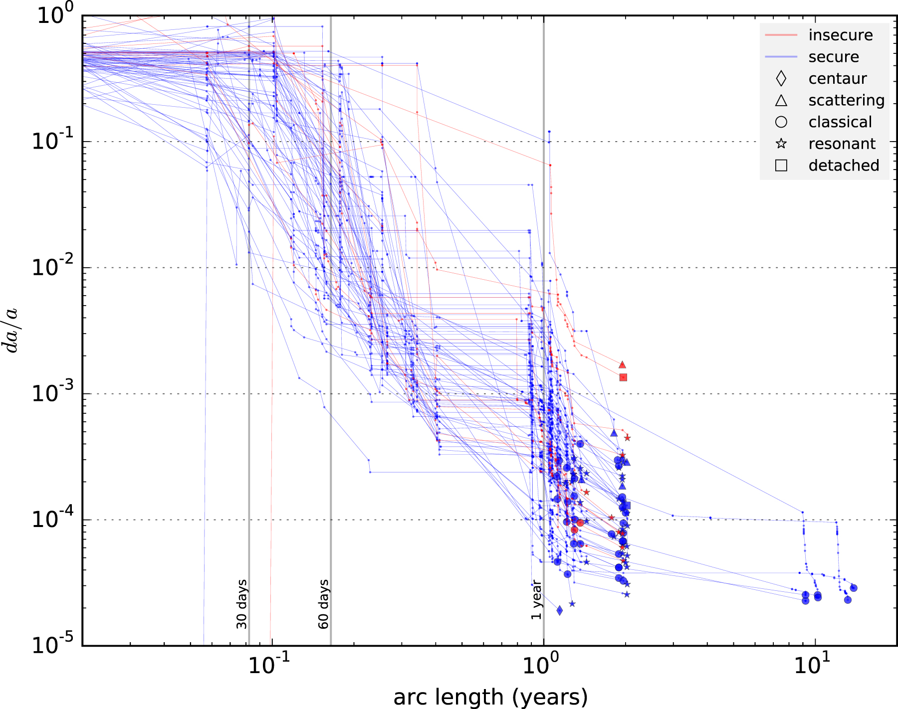