


Abstract
Stellar parameters and abundances have been derived from a sample of 907 F, G, and K dwarfs. The high-resolution, high signal-to-noise spectra utilized were acquired with the HARPS spectrograph of the European Southern Observatory. The stars in the sample with −0.2 < [Fe/H] < +0.2 have abundances that strongly resemble that of the Sun, except for the lithium content and the lanthanides. Near the solar temperature, stars show two orders of magnitude range in lithium content. The average content of stars in the local region appears to be enhanced at about the +0.1 level relative to the Sun for the lanthanides. There are over 100 planet hosts in this sample, and there is no discernible difference between them and the non-hosts regarding their lithium content.
Export citation and abstract BibTeX RIS
1. Introduction
The chemical composition of the local region around the Sun is of vital importance in understanding the history of the elements within the Milky Way. While the Sun often serves as the basis point for abundances, it is necessary to compare those abundances to the mean value and to the dispersion found for local stars. Local in this sense is taken to mean falling within a radius of about 100 pc. The expectation is that the Sun is typical of its neighborhood, but this assumption must be verified. In fact, it is known that there are metal-poor dwarfs in the local region and that abundance trends exist as a function of [Fe/H] in the local stars (for examples, see Luck 2015, 2017). The task is to quantify the range of abundances and the trends within the abundances so that chemical evolution models will have a realistic and reliable end-point target. This paper is the third in a series that has previously considered local giants (Luck 2015) and dwarfs (Luck 2017, hereafter L2017). This paper extends the dwarf sample by analyzing a set of mostly southern dwarfs from archived high-resolution, high signal-to-noise spectra obtained with the HARPS spectrograph at the 3.6 m telescope of the European Southern Observatory.
The rationale for extending the analysis of L2017 is that systematic effects between abundance studies can vitiate zero points in abundances and obscure trends. Systematic effects can include differences in effective temperature scales, offsets in gravity determinations, as well as dissimilarities in atomic data. The better way to overcome these problems is to assemble a large sample of similarly analyzed stars. While the hope is to eliminate systemic effects, the reality is that large samples often reveal previously unsuspected problems in abundance analyses. Given that L2017 is a primarily northern survey, the decision was made to extend the analysis to the southern sky using data from the HARPS spectrograph. This choice is predicated upon data quantity, quality, availability, and overlap with L2017. It was recognized that there would also be a significant commonality with a number of abundance studies of HARPS data, and in particular with those that make use of the data from the HARPS GTO search for Jupiter-mass planets. These analyses are ongoing, with the latest results being found in Suárez-Andrés et al. (2017). Those studies use a different technique for parameter determination from the one used here, and thus intercomparison of the results provides vital information about the reliability of the methodology. Moreover, this work uses data not from the HARPS GTO project(s) mentioned above, and thus contributes comparison abundances for other projects. Lastly, the sample used here contains 140 stars without previous abundance analyses.
For this study, the ESO Archive was searched for dwarfs with HARPS data. The method used was essentially brute force. All reduced HARPS spectra were downloaded, and the objects identified as to type: i.e., dwarf, giant, or other according to the spectral type or parallax information found in SIMBAD. Then, the highest signal-to-noise usable spectra with S/N > 75 was located for each dwarf. This process yielded 907 dwarfs, of which all but one are Hipparcos stars. Of these stars, 128 are planet hosts (Exoplanets team 2017), and 142 are found in L2017. The abundance sample for the HARPS GTO planet-search project is defined in its entirety in Adibekyan et al. (2012). Of the 1111 stars found there, 494 of them are included herein. Basic information about the sample can be found in Table 1. One of the objects analyzed, the Sun, is not found in Table 1.
Table 1. Program Stars
| Primary | HD | HIP | HR | CCDM | Cluster | Spectral Type | P | e_P | V | RV | e_RV | V sin (i) | d | E(B − V) | Mv | Host |
|---|---|---|---|---|---|---|---|---|---|---|---|---|---|---|---|---|
| (mas) | (mas) | (mag) | (km s−1) | (km s−1) | (km s−1) | (pc) | (mag) | (mag) | ||||||||
| V* AH Lep | 36869 | ⋯ | ⋯ | ⋯ | ⋯ | G2V | 28.6 | 7.10 | 8.363 | 24.1 | 2 | 35.0 | 0.000 | 5.64 | ⋯ | |
| *36 Oph B | 155885 | ⋯ | 6401 | J17155–2635B | ⋯ | K1V | 167.1 | 1.10 | 5.08 | ⋯ | ⋯ | 3.7 | 6.0 | 0.000 | 6.19 | ⋯ |
| HD 224789 | 224789 | 57 | ⋯ | ⋯ | ⋯ | K1V | 33.48 | 0.66 | 8.24 | 36.4 | 0.3 | ⋯ | 29.9 | 0.000 | 5.86 | ⋯ |
| HD 224817 | 224817 | 80 | ⋯ | ⋯ | ⋯ | G2V | 13.68 | 1.22 | 9.113 | −11.644 | 0.421 | ⋯ | 73.1 | 0.000 | 4.79 | ⋯ |
| HD 225297 | 225297 | 413 | ⋯ | ⋯ | ⋯ | G0V | 19.51 | 0.63 | 7.74 | 4.7 | 0.3 | ⋯ | 51.3 | 0.000 | 4.19 | ⋯ |
| HD 55 | 55 | 436 | ⋯ | ⋯ | ⋯ | K4.5V | 62.94 | 0.71 | 8.485 | 41 | 2 | ⋯ | 15.9 | 0.000 | 7.48 | ⋯ |
| HD 105 | 105 | 490 | ⋯ | ⋯ | ⋯ | G0V | 25.39 | 0.59 | 7.53 | 1.7 | 0.48 | 14.5 | 39.4 | 0.000 | 4.55 | ⋯ |
| HD 142 | 142 | 522 | 6 | J00063–4905AB | ⋯ | F7V | 38.89 | 0.37 | 5.7 | 6 | 0.53 | 9.34 | 25.7 | 0.000 | 3.65 | H |
| HD 208 | 208 | 569 | ⋯ | ⋯ | ⋯ | G1V | 18.25 | 0.72 | 8.19 | −27.81 | 0.19 | 2.59 | 54.8 | 0.000 | 4.50 | ⋯ |
| HD 283 | 283 | 616 | ⋯ | ⋯ | ⋯ | G9.5V | 30.26 | 1.05 | 8.7 | −42.994 | 0.0043 | ⋯ | 33.0 | 0.000 | 6.10 | ⋯ |
| HD 361 | 361 | 669 | ⋯ | ⋯ | ⋯ | G1V | 36.44 | 0.59 | 7.03 | 7.7 | 0.3 | 2.96 | 27.4 | 0.000 | 4.84 | ⋯ |
| ⋮ | ⋮ | ⋮ | ⋮ | ⋮ | ⋮ | ⋮ | ⋮ | ⋮ | ⋮ | ⋮ | ⋮ | ⋮ | ⋮ | ⋮ | ⋮ | ⋮ |
Note. Information in the first 13 columns is from SIMBAD. CCDM is the Catalog of Double and Multiple Stars. P = parallax in milliarcseconds; source is Hipparcos only. e_P = error in parallax in milliarcseconds. RV = radial velocity in km s−1. e_RV = error in radial velocity in km s−1. V sin (i) = literature-derived projected rotation velocity in km s−1. V = Johnson V apparent magnitude. d = distance in parsecs. E(B − V) = B − V color excess computed from the extinction method of Hakkila et al. (1997); except for d < 75 pc, the extinction is set to 0. Mv = Johnson V-band absolute magnitude. Host = planet-host status—H = known host. The source is The Extrasolar Planets Encyclopedia (Exoplanets team 2017).
Only a portion of this table is shown here to demonstrate its form and content. A machine-readable version of the full table is available.
Download table as: DataTypeset image
2. Observational Material
The spectra used in this work are from the HARPS spectrograph (Mayor et al. 2003) located on the 3.6 m telescope of the European Southern Observatory. The data were obtained in the period 2003–2015, and are drawn from over 140 observing programs. HARPS spectra have a resolution of 115,000 and are continuous over the wavelength range 400–680 nm. The ESO Archive provides the pipeline-reduced spectra used in this analysis. In addition to the dwarf program spectra, a number of high signal-to-noise B star spectra were acquired for use as terrestrial division stars. In all, about 1000 spectra were processed in the course of the analysis. The minimum signal-to-noise utilized was 75, and the median of the average per spectrum signal-to-noise is 130 with a range from 75 to 554. The peak signal-to-noise values are higher, with a median of 213 and a range of 100–663.
The HARPS pipeline wavelength scale is solar system barycentric. However, since the reduction used here performs a terrestrial line cancellation through a B star division, it is necessary to place the spectra back onto the terrestrial wavelength scale using the ESO header-provided barycentric velocity. After this, the spectra are reduced using the ASP spectrum reduction package. This package was written and is maintained by the author. The spectra are first cleaned of cosmic-ray strikes, and the B star division is then performed. The continuum level is set using the interactive graphics continuum-setting subprocess of ASP. The level is determined by visual inspection in 24 nm spectrum sections and placed by the user using straight line segments. The segments can be set arbitrarily by the user or can be guided by polynomial fits of order up to 10. The photospheric wavelength shift relative to the terrestrial scale is determined during the continuum-setting process.
The equivalent-width determination procedure used is described in detail in L2017. The model used is a linear combination of a Gaussian and an exponential profile. The intent is to better account for the line wings. There are free parameters in the fit that relate to the relative contribution of the two profiles and the FWHM of the observed profile. These parameters are functions of the spectrograph resolution, the broadening velocity of the star, and the quickly measured Gaussian equivalent width. The dependence on the broadening velocity means that this parameter must be determined before the equivalent widths can be measured. The broadening velocity is determined by synthesizing the relatively unblended region from 570 to 580 nm. The process is to compute a series of spectra assuming different broadening velocities. In these syntheses, the oscillator strength is used as the free parameter to match the observed depths. A χ2 minimization determines the broadening velocity.
Twenty-five program stars have two measured spectra while two have three measured spectra. The Sun was observed using the Moon and Vesta as reflectors. Comparison of the equivalent widths of lines with values greater than 0.002 nm shows good agreement between the spectra with no systematic effects noted. Most stars have a mean fractional difference (range/mean) of order 0.03–0.05, with the value decreasing toward greater equivalent widths on a per star basis. As expected, lower signal-to-noise spectra show more substantial fractional differences. If more than one spectrum is available, the equivalent width value utilized in the analysis is the simple average.
3. Analysis
3.1. Procedures and Resources
This analysis uses the same procedures and resources as described in detail in Luck (2015, 2017). The basic features are:
- 1.Local thermodynamic equilibrium is assumed.
- 2.Effective temperatures were derived using photometry gleaned from SIMBAD, the Paunzen (2015) uvby compilation, and the General Catalog of Photometric Data (Mermilliod et al. 1997) combined with the color–temperature relations of Casagrande et al. (2010). The reddening was computed from the extinction model of Hakkila et al. (1997), or if the distance is less than 75 pc, it is assumed to be 0 (Vergely et al. 1998; Leroy 1999; Sfeir et al. 1999; Breitschwerdt et al. 2000; Lallement et al. 2003). The metallicity used in the calibration was from either L2017, Bensby et al. (2014), the median value from SIMBAD, an [Fe/H] ratio derived from Strömgren photometry using the Martell & Laughlin (2002) calibration, or assumed solar, in this order of preference.
- 3.Masses and ages are derived using the method of Allende Prieto & Lambert (1999). The isochrones used are from Bertelli et al. (1994), Demarque et al. (2004), Dotter et al. (2008), and the BaSTI Team (2016). The assumed metallicities are the same as those used for the effective temperatures. Gravities are then derived from the mean mass. If the mass is not determinable from the isochrones procedure, the mass is taken from the mean-mass–effective-temperature relation given by the determined masses.
- 4.The line list is that described in detail in Luck (2014, 2017). The oscillator strengths are from an inverted solar analysis using as solar abundances for Z > 10 the values given by Scott et al. (2015a, 2015b) and Grevesse et al. (2015). Damping constants are from Barklem et al. (2000), Barklem & Aspelund-Johanson (2005), or are computed using the Unsöld approximation (Unsöld 1938).
- 5.
- 6.All model stellar atmospheres are plane-parallel MARCS models (Gustafsson et al. 2008). Models at the required parameters and nearest grid metallicity were interpolated using an author-developed code. The grid spacing at metallicities above [M/H] = −1 is 0.25 dex. Given this grid spacing, all models are generally within 0.125 dex in metallicity of the derived value. The line analysis codes are siblings of the MOOG code (Sneden 1973) maintained by the author since 1975.
The rationale behind the use of photometry and isochrones for parameter determination lies in the consideration of a number of factors. The "gold" standard for effective temperatures is the infrared-flux method (IRFM). Although excitation analysis of Fe i lines can yield effective temperatures that reproduce the overall scale of the IRFM, there exists considerable scatter in the derived temperatures. For example, the comparison of the excitation temperatures of Sousa et al. (2008, 2011a, 2011b) with the Casagrande et al. (2010) IRFM temperatures yields a mean temperature difference of −25 K (Casagrande–Sousa); however, the differences range from −371 to 309 K. The position adopted here is that photometrically derived temperatures will reproduce the IRFM temperature scale with less noise than found in excitation temperatures. The stars of this study are relatively bright, and thus have colors available in multiple systems that have an IRFM-based color–temperature calibration. The calibrations used here are from Casagrande et al. (2010). Although multiple photometry sources and systems are used to determine the temperature, the photometric systems utilized are all calibrated using the same standard stars. Additionally, multiple colors yield multiple temperature estimates, allowing outliers to be identified and eliminated. This procedure has been shown to yield high-quality effective temperatures (Luck 2015, 2017).
Gravity determination by isochrone-derived masses has been shown to give gravities that agree well with ionization balance gravities for both giants and dwarfs (Luck 2015, 2017). Using isochrone-derived masses eliminates difficulties from possible non-LTE effects and from blending problems that strongly perturb Fe ii equivalent widths with decreasing temperature.
Tables 2 through 6 contain the results of the analysis. Table 2 presents the effective temperature, mass, and age data along with the calculated gravity. Table 3 has all of the stellar parameters, including the microturbulent and total broadening velocities. Forcing neutral iron line abundances to show no dependence on line strength determines the microturbulent velocity. Also in Table 3 are the details of the Fe i and Fe ii abundances—the mean abundance, standard deviation, and number of lines for each species. Table 4 has the mean [x/H] abundance for each element, and Table 5 has the details of the Li, C, and O analysis. Table 6, whose content is available in machine-readable version, has the details of the abundances for Z > 10—the mean abundance, standard deviation, and number of lines for each species analyzed. The [x/H] ratios of Table 4 are based on the solar abundances determined in this study and presented in Table 6. The Table 4 values for elements with both neutral and first-ionized species are computed as  , where A is the abundance of the element in question, "I" refers to the neutral species, "II" to the first-ionized species, and n is the number of lines. The tables include all stars considered in the analysis: no deletions based on temperature or total broadening have been made in the data presented in table form.
Table 2. Effective Temperature, Mass, and Age Data
| Bertelli | Dartmouth | Yale | BaSTI | |||||||||||||||
|---|---|---|---|---|---|---|---|---|---|---|---|---|---|---|---|---|---|---|
| Primary | T | Sigma | N | log L/Ls | Mass | Age | Mass | Age | Mass | Age | Mass | Age |

|
Range |

|
Range | Mass | log g |
| (K) | (K) | (Ms) | (Gyr) | (Ms) | (Gyr) | (Ms) | (Gyr) | (Ms) | (Gyr) | (Ms) | (Ms) | (Gyr) | (Gyr) | (Ms) | (cm s−2) | |||
| HD 196877 | 4174 | 66 | 12 | −1.12 | ⋯ | ⋯ | ⋯ | ⋯ | 0.58 | 0.60 | 0.56 | 5.29 | 0.57 | 0.02 | 2.95 | 4.69 | 0.57 | 4.74 |
| HD 35650 | 4269 | 47 | 13 | −0.91 | 0.69 | 5.36 | 0.68 | 2.85 | 0.67 | 11.50 | 0.69 | 5.29 | 0.68 | 0.02 | 6.25 | 8.65 | 0.68 | 4.65 |
| HD 118100 | 4308 | 83 | 13 | −0.93 | 0.70 | 0.63 | ⋯ | ⋯ | 0.68 | 4.70 | 0.66 | 5.29 | 0.68 | 0.04 | 3.54 | 4.66 | 0.68 | 4.68 |
| HD 120036 | 4323 | 46 | 3 | −1.07 | ⋯ | ⋯ | ⋯ | ⋯ | ⋯ | ⋯ | ⋯ | ⋯ | ⋯ | ⋯ | ⋯ | ⋯ | 0.68 | 4.83 |
| HD 25004 | 4354 | 36 | 12 | −0.88 | 0.70 | 5.36 | 0.70 | 1.75 | 0.69 | 9.50 | 0.70 | 5.54 | 0.70 | 0.01 | 5.54 | 7.75 | 0.70 | 4.66 |
| HD 93380 | 4359 | 79 | 12 | −0.91 | ⋯ | ⋯ | ⋯ | ⋯ | ⋯ | ⋯ | 0.61 | 10.75 | 0.61 | 0.00 | 10.75 | 0.00 | 0.61 | 4.64 |
| HD 218511 | 4361 | 36 | 9 | −0.82 | 0.73 | 5.36 | 0.68 | 10.25 | ⋯ | ⋯ | ⋯ | ⋯ | 0.71 | 0.05 | 7.81 | 4.89 | 0.71 | 4.61 |
| HD 154363 | 4373 | 42 | 13 | −0.86 | 0.71 | 5.36 | 0.70 | 2.29 | ⋯ | ⋯ | ⋯ | ⋯ | 0.71 | 0.01 | 3.83 | 3.07 | 0.71 | 4.66 |
| V* AO Men | 4384 | 59 | 5 | −0.59 | ⋯ | ⋯ | ⋯ | ⋯ | ⋯ | ⋯ | ⋯ | ⋯ | ⋯ | ⋯ | ⋯ | ⋯ | 0.69 | 4.38 |
| HD 192961 | 4399 | 38 | 12 | −0.82 | 0.70 | 10.07 | 0.70 | 6.45 | ⋯ | ⋯ | ⋯ | ⋯ | 0.70 | 0.00 | 8.26 | 3.62 | 0.70 | 4.62 |
| ⋮ | ⋮ | ⋮ | ⋮ | ⋮ | ⋮ | ⋮ | ⋮ | ⋮ | ⋮ | ⋮ | ⋮ | ⋮ | ⋮ | ⋮ | ⋮ | ⋮ | ⋮ | ⋮ |
| Notes: | Column | Unit | Description | |||||||||||||||
| T | K | Effective Temperature | ||||||||||||||||
| Sig | N/A | Standard deviation of the effective temperature | ||||||||||||||||
| N | N/A | Number of colors used in the effective temperature determination | ||||||||||||||||
| log L/Ls | Solar | Luminosity in logarithmic solar units | ||||||||||||||||
| Bertelli | Mass | Solar | Mass in solar units, determined from the Bertelli et al. (1994) isochrones | |||||||||||||||
| Age | Gyr | Age in gigayears, determined from the Bertelli et al. (1994) isochrones | ||||||||||||||||
| Dartmouth | Mass | Solar | Mass in solar units, determined from the Dotter et al. (2008) isochrones | |||||||||||||||
| Age | Gyr | Age in gigayears, determined from the Dotter et al. (2008) isochrones | ||||||||||||||||
| Yale | Mass | Solar | Mass in solar units, determined from the Demarque et al. (2004) isochrones | |||||||||||||||
| Age | Gyr | Age in gigayears, determined from the Demarque et al. (2004) isochrones | ||||||||||||||||
| BaSTI | Mass | Solar | Mass in solar units, determined from the BaSTI Team (2016) isochrones | |||||||||||||||
| Age | Gyr | Age in gigayears, determined from the BaSTI Team (2016) isochrones | ||||||||||||||||

|
Solar | Average mass in solar masses | ||||||||||||||||
| Range | Solar | Range in mass determination | ||||||||||||||||

|
Gyr | Average age in gigayears | ||||||||||||||||
| Range | Gyr | Range in age determination | ||||||||||||||||
| Mass | Solar | Adopted mass. If  is present, it is that value. For stars with no is present, it is that value. For stars with no  , mass determined from the effective temperature– , mass determined from the effective temperature– relation relation |
||||||||||||||||
| log g | cm s−2 | Surface acceleration, computed from mass, temperature, and luminosity | ||||||||||||||||
Only a portion of this table is shown here to demonstrate its form and content. A machine-readable version of the full table is available.
Table 3. Parameter and Iron Data
| Primary | T | G | Vt | Vb | Fe i | Sigma | N | Fe ii | Sigma | N | [Fe/H] |
|---|---|---|---|---|---|---|---|---|---|---|---|
| (K) | (cm s−2) | (km s−1) | (km s−1) | (log ε) | (log ε) | ||||||
| HD 196877 | 4174 | 4.74 | 0.50 | 2.9 | 6.95 | 0.11 | 160 | 6.85 | 0.39 | 2 | −0.52 |
| HD 35650 | 4269 | 4.65 | 0.50 | 4.8 | 7.50 | 0.15 | 309 | 8.08 | 0.29 | 16 | 0.06 |
| HD 118100 | 4308 | 4.68 | 0.50 | 10.1 | 7.74 | 0.15 | 239 | 7.84 | 0.13 | 4 | 0.27 |
| HD 120036 | 4323 | 4.83 | 0.40 | 2.9 | 7.30 | 0.13 | 196 | 7.31 | 0.31 | 5 | −0.17 |
| HD 25004 | 4354 | 4.66 | 0.50 | 2.7 | 7.42 | 0.06 | 198 | 7.82 | 0.17 | 16 | −0.02 |
| HD 93380 | 4359 | 4.64 | 0.50 | 1.7 | 6.85 | 0.10 | 297 | 7.29 | 0.36 | 22 | −0.59 |
| HD 218511 | 4361 | 4.61 | 0.50 | 3.0 | 7.39 | 0.08 | 122 | 7.33 | 0.09 | 3 | −0.09 |
| HD 154363 | 4373 | 4.66 | 1.00 | 1.7 | 6.82 | 0.11 | 58 | 7.09 | 0.20 | 10 | −0.61 |
| V* AO Men | 4384 | 4.38 | 0.50 | 16.6 | 7.71 | 0.15 | 124 | 7.77 | ⋯ | 1 | 0.24 |
| HD 192961 | 4399 | 4.62 | 1.20 | 1.9 | 7.11 | 0.10 | 163 | 7.54 | 0.31 | 26 | −0.30 |
| ⋮ | ⋮ | ⋮ | ⋮ | ⋮ | ⋮ | ⋮ | ⋮ | ⋮ | ⋮ | ⋮ | ⋮ |
| Column | Column | ||||||||||
| Count | Name | Unit | Description | ||||||||
| 1 | Primary | Primary ID as given by SIMBAD | |||||||||
| 2 | T | K | Effective temperature | ||||||||
| 3 | G | cm s−2 | Logarithm of the surface acceleration (gravity) computed from average mass, temperature, and luminosity | ||||||||
| 4 | Vt | km s−1 | Microturbulent velocity | ||||||||
| 5 | Vb | km s−1 | Broadening velocity assumed to be rotation profile | ||||||||
| 6 | Fe i | log ε | Total iron abundance computed from neutral iron lines. The solar iron abundance is 7.47. | ||||||||
| 7 | Sigma | Standard deviation of the neutral iron line abundances | |||||||||
| 8 | N | Number of neutral iron lines used | |||||||||
| 9 | Fe ii | log ε | Total iron abundance computed from first-ionization stage iron lines. The solar iron abundance is 7.47. | ||||||||
| 10 | Sigma | Standard deviation of the first-ionization stage iron line abundances | |||||||||
| 11 | N | Number of first-ionization stage iron lines used | |||||||||
| 12 | [Fe/H] | Solar | Logarithmic iron abundance relative to the Sun = ((N i * Fe i) + (N ii * Fe ii))/(N i + N ii) − 7.47, where N i = column 8, Fe i = column 7, N ii = column 11, and Fe ii = column 10. | ||||||||
Only a portion of this table is shown here to demonstrate its form and content. A machine-readable version of the full table is available.
Download table as: DataTypeset image
Table 4. [x/H] for Z > 10
| Primary | T | G | Vt | Vb | Na | Mg | Al | Si | S | Ca | Sc | Ti | V | Cr | Mn | Fe | Co | Ni | Cu | Zn | Sr | Y | Zr | Ba | La | Ce | Nd | Sm | Eu |
|---|---|---|---|---|---|---|---|---|---|---|---|---|---|---|---|---|---|---|---|---|---|---|---|---|---|---|---|---|---|
| HD 196877 | 4174 | 4.74 | 0.50 | 2.9 | −0.34 | −0.25 | −0.20 | 0.74 | 1.91 | 0.19 | 0.08 | −0.28 | 0.06 | −0.22 | −0.52 | −0.52 | 0.05 | −0.05 | −0.34 | 0.53 | −0.12 | −0.34 | −0.50 | −0.57 | 0.35 | 0.27 | 0.52 | 0.10 | 0.47 |
| HD 35650 | 4269 | 4.65 | 0.50 | 4.8 | −0.11 | 0.05 | −0.06 | 0.51 | 1.61 | 0.32 | 0.10 | 0.01 | 0.25 | 0.08 | −0.02 | 0.06 | 0.19 | 0.17 | 0.03 | 0.71 | 0.27 | 0.06 | 0.10 | 0.00 | 0.62 | 0.61 | 0.64 | 0.52 | 0.42 |
| HD 118100 | 4308 | 4.68 | 0.50 | 10.1 | 0.00 | 0.20 | −0.02 | 0.67 | 1.83 | 0.11 | 0.45 | 0.14 | 0.39 | 0.34 | 0.16 | 0.27 | 0.34 | 0.33 | 0.29 | 0.42 | 0.13 | 0.25 | 0.19 | 0.69 | 0.46 | 1.09 | 0.87 | ||
| HD 120036 | 4323 | 4.83 | 0.40 | 2.9 | −0.12 | −0.07 | −0.07 | 0.54 | 1.44 | 0.49 | 0.28 | 0.04 | 0.27 | 0.04 | −0.14 | −0.17 | 0.26 | 0.09 | −0.16 | −0.07 | 0.23 | −0.04 | 0.13 | −0.15 | 0.55 | 0.39 | 0.85 | 0.52 | 0.58 |
| HD 25004 | 4354 | 4.66 | 0.50 | 2.7 | −0.14 | −0.05 | −0.15 | 0.22 | 1.05 | 0.15 | 0.05 | −0.09 | 0.17 | −0.01 | −0.19 | −0.03 | 0.07 | 0.04 | −0.18 | 0.05 | −0.01 | −0.18 | 0.14 | −0.13 | 0.32 | 0.23 | 0.65 | 0.43 | 0.41 |
| HD 93380 | 4359 | 4.64 | 0.50 | 1.7 | −0.55 | −0.55 | −0.51 | −0.07 | 0.69 | −0.29 | −0.40 | −0.51 | −0.34 | −0.50 | −0.70 | −0.59 | −0.23 | −0.46 | −0.58 | −0.34 | −0.45 | −0.87 | −0.40 | −0.81 | −0.20 | −0.28 | 0.22 | −0.07 | |
| HD 218511 | 4361 | 4.61 | 0.50 | 3.0 | 0.02 | 0.13 | 0.06 | 0.36 | 1.25 | 0.29 | 0.22 | 0.01 | 0.31 | 0.10 | −0.06 | −0.09 | 0.16 | 0.15 | 0.00 | 0.32 | 0.09 | −0.15 | 0.17 | −0.25 | 0.56 | 0.24 | 0.63 | 0.50 | 0.33 |
| HD 154363 | 4373 | 4.66 | 1.00 | 1.7 | −0.42 | −0.18 | −0.18 | 0.17 | 1.05 | −0.02 | −0.12 | −0.31 | −0.15 | −0.42 | −0.66 | −0.61 | −0.09 | −0.26 | −0.33 | −0.19 | −0.35 | −0.53 | −0.47 | −0.83 | 0.19 | 0.09 | 0.18 | 0.02 | 0.28 |
| V* AO Men | 4384 | 4.38 | 0.50 | 16.6 | 0.13 | 0.25 | −0.15 | 0.45 | 1.25 | 0.17 | 0.21 | 0.14 | 0.21 | 0.40 | 0.14 | 0.24 | 0.53 | 0.36 | 0.45 | 0.53 | 0.30 | −0.09 | 0.43 | 1.67 | 0.78 | ||||
| HD 192961 | 4399 | 4.62 | 1.20 | 1.9 | −0.18 | −0.17 | −0.16 | 0.15 | 0.89 | −0.09 | −0.15 | −0.32 | −0.05 | −0.21 | −0.30 | −0.30 | −0.08 | −0.12 | −0.30 | −0.10 | −0.26 | −0.54 | −0.43 | −0.63 | 0.03 | −0.16 | 0.22 | −0.10 | 0.14 |
| ⋮ | ⋮ | ⋮ | ⋮ | ⋮ | ⋮ | ⋮ | ⋮ | ⋮ | ⋮ | ⋮ | ⋮ | ⋮ | ⋮ | ⋮ | ⋮ | ⋮ | ⋮ | ⋮ | ⋮ | ⋮ | ⋮ | ⋮ | ⋮ | ⋮ | ⋮ | ⋮ | ⋮ | ⋮ | ⋮ |
| Column | Units | Designation | Description | ||||||||||||||||||||||||||
| Primary | Primary ID as given by SIMBAD | ||||||||||||||||||||||||||||
| T | K | Teff | Effective temperature | ||||||||||||||||||||||||||
| G | cm s−1 | log g | log of the surface acceleration due to gravity | ||||||||||||||||||||||||||
| Vt | km s−1 | Vt | Microturbulent velocity | ||||||||||||||||||||||||||
| Vr | km s−1 | Vr | Broadening velocity assumed to be rotation profile | ||||||||||||||||||||||||||
| Na | Solar | [Na/H] | Abundance of sodium given logarithmically with respect to the solar value | ||||||||||||||||||||||||||
| Mg | Solar | [Mg/H] | Abundance of magnesium given logarithmically with respect to the solar value | ||||||||||||||||||||||||||
| Al | Solar | [Al/H] | Abundance of aluminum given logarithmically with respect to the solar value | ||||||||||||||||||||||||||
| Si | Solar | [Si/H] | Abundance of silicon given logarithmically with respect to the solar value | ||||||||||||||||||||||||||
| S | Solar | [S/H] | Abundance of sulfur given logarithmically with respect to the solar value | ||||||||||||||||||||||||||
| Ca | Solar | [Ca/H] | Abundance of calcium given logarithmically with respect to the solar value | ||||||||||||||||||||||||||
| Sc | Solar | [Sc/H] | Abundance of scandium given logarithmically with respect to the solar value | ||||||||||||||||||||||||||
| Ti | Solar | [Ti/H] | Abundance of titanium given logarithmically with respect to the solar value | ||||||||||||||||||||||||||
| V | Solar | [V/H] | Abundance of vanadium given logarithmically with respect to the solar value | ||||||||||||||||||||||||||
| Cr | Solar | [Cr/H] | Abundance of chromium given logarithmically with respect to the solar value | ||||||||||||||||||||||||||
| Mn | Solar | [Mn/H] | Abundance of manganese given logarithmically with respect to the solar value | ||||||||||||||||||||||||||
| Fe | Solar | [Fe/H] | Abundance of iron given logarithmically with respect to the solar value | ||||||||||||||||||||||||||
| Co | Solar | [Co/H] | Abundance of cobalt given logarithmically with respect to the solar value | ||||||||||||||||||||||||||
| Ni | Solar | [Ni/H] | Abundance of nickel given logarithmically with respect to the solar value | ||||||||||||||||||||||||||
| Cu | Solar | [Cu/H] | Abundance of copper given logarithmically with respect to the solar value | ||||||||||||||||||||||||||
| Zn | Solar | [Zn/H] | Abundance of zinc given logarithmically with respect to the solar value | ||||||||||||||||||||||||||
| Sr | Solar | [Sr/H] | Abundance of strontium given logarithmically with respect to the solar value | ||||||||||||||||||||||||||
| Y | Solar | [Y/H] | Abundance of yttrium given logarithmically with respect to the solar value | ||||||||||||||||||||||||||
| Zr | Solar | [Zr/H] | Abundance of zirconium given logarithmically with respect to the solar value | ||||||||||||||||||||||||||
| Ba | Solar | [Ba/H] | Abundance of barium given logarithmically with respect to the solar value | ||||||||||||||||||||||||||
| La | Solar | [La/H] | Abundance of lanthanum given logarithmically with respect to the solar value | ||||||||||||||||||||||||||
| Ce | Solar | [Ce/H] | Abundance of cerium given logarithmically with respect to the solar value | ||||||||||||||||||||||||||
| Nd | Solar | [Nd/H] | Abundance of neodymium given logarithmically with respect to the solar value | ||||||||||||||||||||||||||
| Sm | Solar | [Sm/H] | Abundance of samarium given logarithmically with respect to the solar value | ||||||||||||||||||||||||||
| Eu | Solar | [Eu/H] | Abundance of europium given logarithmically with respect to the solar value. | ||||||||||||||||||||||||||
Note.
Abundances with both neutral and ionized species are calculated thus:  , where "I" refers to the neutral species, "II" to the first-ionized species, n to the number of lines, and A to the abundance. The number of lines and abundances are given in Table 6.
The solar abundances used to calculate [x/H] are those given in Table 6. They were determined using reflection spectra of the Moon and Vesta.
Only a portion of this table is shown here to demonstrate its form and content. A machine-readable version of the full table is available.
Table 5. Lithium, Carbon, and Oxygen Data
| Primary | T | G | Vt | Vb | [Fe/H] | Li | NLTE | L | 505.20 | 538.00 | C2 | 615.50 | 630.00 |

|

|
[C/H] | [O/H] | [C/Fe] | [O/Fe] |
|---|---|---|---|---|---|---|---|---|---|---|---|---|---|---|---|---|---|---|---|
| (K) | (cm s−2) | (km s−1) | (km s−1) | (log ε) | (log ε) | (log ε) | (log ε) | (log ε) | (log ε) | (log ε) | (log ε) | ||||||||
| HD 196877 | 4174 | 4.74 | 0.50 | 2.9 | −0.52 | −0.02 | 0.17 | ⋯ | ⋯ | ⋯ | ⋯ | ⋯ | ⋯ | ⋯ | ⋯ | ⋯ | ⋯ | ⋯ | ⋯ |
| HD 35650 | 4269 | 4.65 | 0.50 | 4.8 | 0.06 | 0.04 | 0.18 | ⋯ | ⋯ | ⋯ | 8.94 | ⋯ | 9.27 | 8.93 | 9.27 | 0.50 | 0.58 | 0.44 | 0.51 |
| HD 118100 | 4308 | 4.68 | 0.50 | 10.1 | 0.27 | 0.50 | 0.19 | ⋯ | ⋯ | ⋯ | 8.81 | ⋯ | 9.13 | 8.79 | 9.13 | 0.36 | 0.44 | 0.09 | 0.16 |
| HD 120036 | 4323 | 4.83 | 0.40 | 2.9 | −0.17 | 0.26 | 0.19 | ⋯ | ⋯ | ⋯ | ⋯ | ⋯ | ⋯ | ⋯ | ⋯ | ⋯ | ⋯ | ⋯ | ⋯ |
| HD 25004 | 4354 | 4.66 | 0.50 | 2.7 | −0.02 | 0.13 | 0.19 | ⋯ | ⋯ | ⋯ | 9.08 | ⋯ | 9.28 | 9.06 | 9.28 | 0.63 | 0.59 | 0.65 | 0.61 |
| HD 93380 | 4359 | 4.64 | 0.50 | 1.7 | −0.59 | −0.36 | 0.19 | ⋯ | ⋯ | ⋯ | 8.46 | ⋯ | 8.72 | 8.44 | 8.72 | 0.01 | 0.03 | 0.60 | 0.61 |
| HD 218511 | 4361 | 4.61 | 0.50 | 3.0 | −0.09 | 0.07 | 0.19 | ⋯ | ⋯ | ⋯ | 8.96 | ⋯ | 9.27 | 8.94 | 9.27 | 0.51 | 0.58 | 0.60 | 0.67 |
| HD 154363 | 4373 | 4.66 | 1.00 | 1.7 | −0.61 | −0.17 | 0.19 | ⋯ | ⋯ | ⋯ | 8.65 | ⋯ | 9.09 | 8.63 | 9.09 | 0.20 | 0.40 | 0.82 | 1.01 |
| V* AO Men | 4384 | 4.38 | 0.50 | 16.6 | 0.24 | 3.10 | 0.19 | ⋯ | ⋯ | ⋯ | 8.67 | ⋯ | 8.86 | 8.65 | 8.86 | 0.22 | 0.17 | −0.02 | −0.07 |
| HD 192961 | 4399 | 4.62 | 1.20 | 1.9 | −0.30 | −0.08 | 0.19 | ⋯ | ⋯ | ⋯ | 8.80 | ⋯ | 9.08 | 8.78 | 9.08 | 0.35 | 0.39 | 0.65 | 0.70 |
| ⋮ | ⋮ | ⋮ | ⋮ | ⋮ | ⋮ | ⋮ | ⋮ | ⋮ | ⋮ | ⋮ | ⋮ | ⋮ | ⋮ | ⋮ | ⋮ | ⋮ | ⋮ | ⋮ | ⋮ |
| Primary | Primary ID as given by SIMBAD | ||||||||||||||||||
| T | K | Effective temperature | |||||||||||||||||
| G | cm s−2 | Logarithm of the surface acceleration (gravity) computed from average mass, temperature, and luminosity | |||||||||||||||||
| Vt | km s−1 | Microturbulent velocity | |||||||||||||||||
| Vb | km s−1 | Broadening velocity assumed to be rotation profile | |||||||||||||||||
| Fe | log ε | Iron abundance. The solar iron abundance is 7.47 relative to H = 12. | |||||||||||||||||
| Li | log ε | Lithium abundance. The solar lithium abundance is 1.0 dex. | |||||||||||||||||
| NLTE | Correction for non-local thermodynamic equilibrium | ||||||||||||||||||
| L | L = Upper limit on lithium abundance | ||||||||||||||||||
| 505.2 | log ε | Carbon abundance from the C i 505.2 nm line | |||||||||||||||||
| 538.0 | log ε | Carbon abundance from the C i 538.0 nm line | |||||||||||||||||
| C2 | log ε | Carbon abundance from the C2 Swan lines—primary indicator at 513.5 nm | |||||||||||||||||
| 615.5 | log ε | Oxygen abundance from the [O i] 630.0 nm line | |||||||||||||||||
| 630.0 | log ε | Oxygen abundance from the O i 615.5 triplet | |||||||||||||||||

|
log ε | Mean carbon abundance—weights discussed in text | |||||||||||||||||

|
log ε | Mean oxygen abundance—weights discussed in text | |||||||||||||||||
| [C/H] | Solar | Mean carbon abundance relative to the solar value | |||||||||||||||||
| [O/H] | Solar | Mean oxygen abundance relative to the solar value | |||||||||||||||||
| [C/Fe] | Mean carbon abundance relative to iron in solar units | ||||||||||||||||||
| [O/Fe] | Mean oxygen abundance relative to iron in solar units | ||||||||||||||||||
Only a portion of this table is shown here to demonstrate its form and content. A machine-readable version of the full table is available.
Table 6. log ε Details for Z > 10
| Column | Label | Description |
|---|---|---|
| 1 | Primary | Primary Name for the star |
| 2 | Teff | Effective temperature (K) |
| 3 | Log(g) | Log surface gravity (cm s−2) |
| 4 | Vt | Microturbulent velocity (km s−1) |
| 5 | Vb | Broadening velocity assumed to be rotation profile |
| 6 | log ε | Mean abundance of Na i relative to log ε(hydrogen) = 12 |
| 7 | Sigma | Standard deviation of the abundance about the mean |
| 8 | N | Number of lines used in the mean abundance |
| 9–110 | $⋯$ | Columns 9–110 repeat the Na i sequence for Mg i, Al i, Si i, Si ii, S i, Ca i, Ca ii, Sc i, Sc ii, Ti i, Ti ii, V i, V ii, Cr i, Cr ii, Mn i, Fe i, Fe ii, Co i, Ni i, Cu i, Zn i, Sr i, Y i, Y ii, Zr i, Zr ii, Ba ii, La ii, Ce ii, Pr ii, Nd ii, Sm ii, and Eu ii |
Only a portion of this table is shown here to demonstrate its form and content. A machine-readable version of the full table is available.
Download table as: DataTypeset image
3.2. Parameter and Abundance Inspection
In this section, the various parameters and abundances will be examined for untoward trends, and a comparison with other analyses will also be made. For the program stars, SIMBAD gives 225 individual papers with information on [Fe/H], stellar parameters, or both. It is not possible to consider all of these works. The comparisons made will be to selected works that have significant overlap with the current study, or that are important regarding determining how robust the parameters and abundances determined here are.
3.2.1. Temperature
Table 2 gives the adopted temperature, standard deviation about the mean, and the number of colors used to determine the temperature. The number of colors possible in the temperature determination is 13, with the median number utilized equal to 10. The range in the number of colors utilized is one to thirteen. In combining the individual temperature estimates, it was noted that colors involving the 2MASS magnitudes J and H were often discrepant due to saturation. Therefore, all colors involving J for stars brighter than mV = 7 were eliminated. Similarly, for stars brighter than V = 6, colors involving H were eliminated. The temperature data were individually examined on a per star basis if the standard deviation was greater than 100 K and discrepant estimates eliminated.
The agreement between the various individual temperature estimates is rather good. The standard deviations range from 8 to 99 K with the median standard deviation being 44 K. Looking at the standard deviation as a percentage of the effective temperature, the standard deviation has a maximum value of 2% of the effective temperature and a median value of 0.78%.
The Casagrande et al. (2010) color–temperature relation does have a metallicity dependence. The [Fe/H] ratios used in the calibration are detailed in Section 3.1. Comparison of the final derived [Fe/H] values (see Table 4) with the initial assumptions shows excellent agreement. The mean difference is +0.04 (final [Fe/H] larger) with a standard deviation of 0.15 dex. To test the sensitivity of the color–temperature calibration to metallicity variation, the input metallicity values were varied by ±0.2 dex. The resulting temperature variation is 8 K in the mean with a standard deviation of 11 K. The photometric temperatures derived here thus do not show significant sensitivity to the initial [Fe/H] values as long as that value is reasonable.
In Table 7, mean temperature differences (this work – other works) are given for a variety of studies. It is worth noting that this study reproduces the IRFM effective temperatures of Casagrande et al. (2010) very precisely. Sixty-two stars are in common with a mean difference of only 1 K and a standard deviation of 35 K. Similar differences are found between this study and its predecessor, L2017. The mean difference for the 140 common stars is 1 K with a standard deviation of 17 K. The reason why there is a difference is that while the same photometry and calibration were used in both, the editing of the temperature estimates differed in the handing of the 2MASS-related colors.
Table 7. Parameter and Abundance Comparisons
| Study | N | T type | G type |

|
s_T |

|
s_G |

|
s_Fe |

|
s_C |

|
s_O |
|---|---|---|---|---|---|---|---|---|---|---|---|---|---|
| This versus C+2010 | 62 | IRFM | Var | 1 | 34 | 0.05 | 0.14 | ⋯ | ⋯ | ⋯ | ⋯ | ⋯ | ⋯ |
| This versus C+2011 | 612 | Var | Var | −28 | 53 | −0.01 | 0.05 | 0.04 | 0.16 | ⋯ | ⋯ | ⋯ | ⋯ |
| This versus MM2012 | 14 | Var | A | 34 | 41 | −0.03 | 0.07 | 0.04 | 0.06 | ⋯ | ⋯ | ⋯ | ⋯ |
| This versus A+2012 | 494 | E | Ion | −9 | 68 | −0.01 | 0.15 | 0.02 | 0.05 | ⋯ | ⋯ | ⋯ | ⋯ |
| This versus T+2013 | 350 | E, IRFM | Ion | 19 | 54 | 0.05 | 0.15 | 0.03 | 0.05 | ⋯ | ⋯ | ⋯ | ⋯ |
| This versus C+2013 | 9 | Var | A | 87 | 86 | 0.00 | 0.06 | −0.01 | 0.15 | ⋯ | ⋯ | ⋯ | ⋯ |
| This versus R+2013 | 113 | E | Ion | 8 | 33 | 0.01 | 0.04 | 0.02 | 0.04 | ⋯ | ⋯ | 0.05 | 0.12 |
| This versus R+2014 | 42 | E | Ion | −16 | 41 | −0.05 | 0.04 | 0.01 | 0.02 | 0.00 | 0.05 | 0.02 | 0.06 |
| This versus B+2014 | 163 | E | Ion | 14 | 86 | −0.10 | 0.05 | 0.01 | 0.05 | ⋯ | ⋯ | 0.06 | 0.18 |
| This versus B+2015 | 339 | E, IRFM | Ion | 0 | 59 | −0.05 | 0.13 | 0.01 | 0.04 | ⋯ | ⋯ | 0.01 | 0.11 |
| This versus S+2015 | 7 | N | N | 74 | 86 | 0.11 | 0.11 | 0.03 | 0.05 | ⋯ | ⋯ | ⋯ | ⋯ |
| This versus B+2016 | 135 | SME | SME | 10 | 50 | 0.00 | 0.08 | 0.00 | 0.05 | −0.05 | 0.08 | −0.03 | 0.11 |
| This versus L2017 | 140 | P | Iso | 1 | 17 | 0.00 | 0.05 | −0.03 | 0.13 | 0.01 | 0.08 | 0.00 | 0.20 |
| This versus SA+2017 | 494 | E | E | 11 | 63 | 0.00 | 0.17 | 0.02 | 0.05 | 0.02 | 0.12 | ⋯ | ⋯ |
| B+2014 versus A+2012 | 166 | ⋯ | ⋯ | −12 | 56 | −0.08 | 0.15 | −0.02 | 0.05 | ⋯ | ⋯ | ⋯ | ⋯ |
| B+2016 versus A+2012 | 101 | ⋯ | ⋯ | −31 | 61 | −0.01 | 0.11 | 0.02 | 0.05 | ⋯ | ⋯ | ⋯ | ⋯ |
| N | Number of common stars | ||||||||||||
| T Type | Method of effective temperature determination in comparison study. P = Photometric, E = Excitation analysis, IRFM = InfraRed Flux Method, Var = combination or literature derived, SME = Spectroscopy Made Easy (Valenti & Piskunov 1996), N = non-LTE | ||||||||||||
| G Type | Method of gravity determination in comparison study. Iso = Isochrone fit, Ion = spectroscopic ionization balance, Var = Combination (excitation/isochrones/literature), A = astroseismology, SME = Spectroscopy Made Easy (Valenti & Piskunov 1996), N = non-LTE | ||||||||||||
| dT | = New effective temperature – source | ||||||||||||
| dG | = New Gravity – source | ||||||||||||
| dFe | = New [Fe/H] – source | ||||||||||||
| dC | = New mean carbon – source | ||||||||||||
| dO | = New mean oxygen – source | ||||||||||||
| s_X | = Standard deviation of differences | ||||||||||||
| Comparison Studies: | |||||||||||||
| C+2010 | Casagrande et al. (2010) | ||||||||||||
| C+2011 | Casagrande et al. (2011) | ||||||||||||
| MM2012 | Morel & Miglio (2012) | ||||||||||||
| A+2013 | Adibekyan et al. (2012) | ||||||||||||
| A+2013 is the aggregation of parameters from Sousa et al. (2008, 2011a, 2011b) | |||||||||||||
| T+2013 | Tsantaki et al. (2013) | ||||||||||||
| C+2013 | Creevey et al. (2013) | ||||||||||||
| R+2013 | Ramírez et al. (2013) | ||||||||||||
| R+2014 | Ramírez et al. (2014) | ||||||||||||
| B+2014 | Bensby et al. (2014) | ||||||||||||
| B+2015 | Bertran de Lis et al. (2015) | ||||||||||||
| B+2015 takes most of their parameters from Tsantaki et al. (2013) | |||||||||||||
| S+2015 | Sitnova et al. (2015) | ||||||||||||
| B+2016 | Brewer et al. (2016) | ||||||||||||
| L2017 | Luck (2017) using mass-derived gravity | ||||||||||||
| SA+2017 | Suárez-Andrés et al. (2017) | ||||||||||||
The other sources have systematic temperature differences relative to this work that range up to 87 K, with the largest differences in the Creevey et al. (2013) and Sitnova et al. (2015) values. The effective temperatures used by Creevey et al. were taken from previous analyses and thus do not constitute a self-consistent sample. The Sitnova et al. values are self-consistent and were derived from an excitation analysis of Fe i lines using non-LTE level populations. They are thus dependent upon the non-LTE physics, the model atmospheres, and atomic parameters. Another point about the Creevey et al. and Sitnova et al. comparisons is that they involve relatively few stars.
The remaining studies can have over 100 stars in common with the present work. The average difference for those works is in the range 8–35 K. The most common type of effective temperature determination in these cases is a traditional excitation analysis. Overall, the scale agreement between the various studies is adequate. However, the individual effective temperature differences can be large—witness the variation between this work and the Adibekyan et al. (2012) compilation of effective temperatures from Sousa et al. (2008, 2011a, 2011b). The mean difference based on 494 stars is 9 K with a standard deviation of 68 K, but the range is from −350 to 294 K. This behavior indicates that the overall scale is good, but that the scatter is significant. The same is true for all of the excitation analyses. One might think that the fault lies in the photometric temperatures used here, but a comparison of the Bensby et al. (2014) and the Brewer et al. (2016) excitation analysis temperatures to the Adibekyan et al. values indicates similar variations. This result does not absolve the photometric results but does indicate that there are problems in the excitation analyses.
3.2.2. Mass, Age, and Gravity
One of the quantities needed for the determination of stellar abundances is the surface gravity. If the mass, luminosity, and effective temperature are known, the gravity is easily found. This sample has luminosities determined using Hipparcos parallaxes (van Leeuwen 2007), and effective temperatures determined from photometry. Isochrones from four different sources are used to obtain the mass. The mass determined from each source is given in Table 2 along with the age from that isochrone source. Table 2 also gives the spread in mass and age over the isochrone fits. The data are very consistent for the masses. The median mass of the sample is 0.99 solar masses with a total range of 0.57–1.47 solar masses. The median spread for the individual determinations is 0.06 solar masses with a range of the total spread from zero to 0.47 solar masses. The fractional difference is thus about 6%. The uncertainty in the derived gravities due to this mass uncertainty is about ±0.03 dex.
Isochrones are metallicity dependent, and thus the choice of metallicity can affect the derived mass. As given previously in Section 3.2.1, the input metallicity used to derived the temperatures and masses agrees well with the final value. To test the sensitivity of the isochrone-derived masses, the BaSTI isochrones were used to derive masses for the program stars with an offset of −0.2 dex relative to the adopted [Fe/H] value. The masses found varied only by a mean value of 0.03 solar masses with a spread in the difference of 0–0.26 solar masses. The standard deviation of the differences is 0.03 solar masses. A mass change of 0.03 solar masses at constant effective temperature and luminosity translated to a difference of about 0.01 in log g.
One concern in a study such as this is the consistency of the sample selection. In this case, the worry is that some of the stars might not be dwarfs. The selection criterion tries to ensure that the absolute magnitude at a given temperature is appropriate for a dwarf. The total sample is shown in Figure 1 in an HR diagram with the derived effective temperatures versus luminosity (logarithmic) in solar units. Also shown is the ZAMS for solar composition and three mass tracks: 0.75, 1.00, and 1.25 solar masses with maximum ages of 10, 10, and 3 Gyr, respectively. The ZAMS and tracks are from the BaSTI database (BaSTI 2016). Given the actual range and metallicity in the sample, the scatter above the ZAMS is as expected, and the behavior of tracks indicates that these stars are still on or near the main sequence.
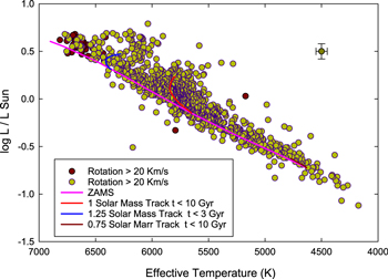
Figure 1. HR diagram of the program stars with the ZAMS and evolutionary tracks (BaSTI 2016) for three masses indicated. The stars with a total broadening velocity of 20 km s−1 or greater are also indicated. Given the spread in metallicity and age, these stars are all dwarfs.
Download figure:
Standard image High-resolution imageAlthough the masses are well determined, the same cannot be said for the ages. The range of the ages has a median value of 2.9 Gyr or about 60% of the median age of 4.9 Gyr. It is important to emphasize that the spreads discussed above are not based upon the uncertainty found from a single isochrone set, but are determined from the differences in the age found from different isochrone sets. It must be emphasized at this point that the ages derived here are not reliable and thus attempts to ascertain age–metallicity relations using these ages are futile.
A common practice for the determination of isochrone-based masses is to adopt a single set of isochrones. Brewer et al. (2016) give masses determined from the Yale isochrones (Demarque et al. 2004). For the common stars, the median difference in mass is 0.013 solar masses for this choice of isochrone. Comparing the Brewer et al. masses to the average isochrone value used here, the median difference is −0.005 solar masses. Overall, the mass comparison is excellent. A median difference of −0.3 Gyr is found between the Brewer et al. ages and those found here, but the variation is significant with differences as large as 11 Gyr noted.
The behavior of the masses and ages reflects the fact that in the isochrones, a relatively narrow range in mass occupies a particular target box in temperature and luminosity. However, that small range in mass can take significantly different evolutionary times to reach the box. These times vary not only because of the differing rates of evolution but also because of different physical assumptions between the isochrone sets, as well as uncertainties due to the chosen metallicity.
Inspection of the gravity differences given in Table 7 indicates that in all cases the surface gravities compare very nicely. The mean differences are of order 0.05–0.11 dex with, in general, relatively small scatter, regardless of whether the source study uses an ionization balance with LTE or non-LTE populations, isochrone masses, or astroseismology. It appears that the various methods are converging on a single answer for the gravity.
3.2.3. Total Broadening Velocity
In Table 3, the total broadening velocity needed to match the line profiles in the program stars is given. The stellar convolution shape assumed here is a rotation profile and a fixed Gaussian macroturbulent velocity of 0.25 km s−1. The computation of the observed stellar profile also requires the spectrograph slit profile. The slit profile was determined from comparison arcs taken with the spectra. Arcs from the total range of dates for the spectroscopic data were utilized, and no significant variation is noted.
Among the target spectra are solar reflection spectra taken using Vesta and the Moon as the reflector. The best-fit total broadening velocity obtained for the Sun is 3.6 km s−1. This velocity is the convolution of macroturbulence and rotation. At low velocities, the total convolution velocity is to first order the Gaussian sum of the two. dos Santos et al. (2016) give the macroturbulent velocity for the Sun to be from 2.9 to 3.6 km s−1, depending on the line, and the rotational velocity to be 2.04 km s−1. Most of the lines they considered have macroturbulent velocities of about 3 km s−1. The total solar broadening velocity is 3.6 km s−1 assuming a macroturbulent velocity of 3 km s−1—exactly the velocity derived here.
Rotational velocities have been published for 505 of the program stars and are presented by SIMBAD (see Table 1). These values are in most cases total broadening velocities. Comparison of the unfiltered literature data to the total broadening velocity derived here indicates a mean offset of 0.2 km s−1 with a standard deviation of 4.7 km s−1. At larger velocities, the literature values can be much higher than those determined here, but given the uncertain quality of many of the literature values, this level of agreement is good.
Brewer et al. (2016) have derived total velocity broadening for a large sample of dwarfs. This study has 135 stars in common with Brewer et al. They assumed a pure Gaussian for their initial fit profile and then went on to "de-convolve" the rotation and macroturbulence. The deconvolution was done by assuming stars with very low total broadening to have no rotation, and they then fit the observed macroturbulent velocities to a power law as a function of temperature. The spectra were then matched with the temperature-derived macroturbulence as a fixed value and using the rotational velocity as the free parameter. For the common stars, the mean difference between the Brewer et al. total broadening velocities and those determined here is −0.5 km s−1 (this study—Brewer et al.) with a standard deviation of 0.7 km s−1.
In Figure 2, the total velocities derived here are shown versus the Brewer et al. total broadening velocity, macroturbulent velocity, and rotation velocity. The low total velocity points dominate the mean differences. At higher velocities, the total velocity values determined here are systematically lower than those determined by Brewer et al. However, the rotational velocities of Brewer et al. match rather well with those determined here if the velocity is greater than about 8 km s−1. An oddity is that there are macroturbulent velocities in the Brewer et al. data that are larger than the corresponding total broadening velocity. An examination of their entire data set finds that 11% of their stars have this property. Figure 3 shows profile matches generated by three choices of broadening parameters: the total broadening used here, the total broadening found by Brewer et al., and the combined Brewer et al. macroturbulent and rotation velocity. The broadening used here provides an excellent fit for these stars, and in general, is not significantly different from that of Brewer et al. In the case of HD 200565, the fit obtained here is superior to either fit generated using the Brewer et al. parameters. Although a better comparison would be heartwarming, an examination of the fits obtained here yield no problems with profile matches.
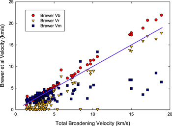
Figure 2. Total broadening velocity determined through spectrum synthesis using a rotation profile vs. the Brewer et al. (2016) total broadening velocity (Vb), rotation (Vr), and the macroturbulent (Vm) components. The straight line is the line of equality. The mean difference is −0.5 km s−1 for the total broadening velocity (Vb). At larger velocities, better agreement is obtained between the Brewer Vr values and the total broadening velocity.
Download figure:
Standard image High-resolution image
Figure 3. Synthesis fits for three stars using different sets of broadening parameters: the total broadening from this study, the Brewer et al. (2016) total broadening, and the combined rotation and macroturbulent velocities. For the top and bottom stars, the syntheses show only minor differences, but for HD 200565, the broadening used here is superior. In the synthesis of HD 90711, another common synthesis problem is evident; the strong Ca i line at 585.74 has mismatched wings due to inaccurate damping constants. The broadening parameters are given as a quartet of velocities in km s−1 in each panel: (This work Vb, Brewer et al. Vb, Brewer et al. macroturbulence, Brewer et al. rotation).
Download figure:
Standard image High-resolution imageThe reliability of the equivalent widths and thus the abundances derived from them determined for this study are a direct function of the broadening velocity. Above a total broadening of 20 km s−1, the equivalent-width determination algorithm fails. In the discussion of the Z > 10 abundances, all stars above this rotation limit will be excluded. The restriction removes 28 stars from the study. Note that in the determination of effective temperatures and surface gravities, the broadening velocity does not enter.
3.2.4. Z > 10 Abundances
The most critical element for Z > 10 is iron. It is often used to characterize the overall metallicity of a star, can be used to determine stellar parameters, and has the greatest statistical presence due to a large number of neutral and ionized lines available in mid-type dwarfs. For this sample, the average number of Fe i lines is 410, and the average for Fe ii is 52. Note that these averages are for lines that were retained after a statistical line culling as described in L2017 was applied: the original numbers are much larger.
In Figure 4, the distribution of Fe i abundances is shown overplotted with the difference Fe i – Fe ii. There is little evidence for systematic behavior in Fe i as a function of temperature, but the difference decreases as the temperature decreases especially once a temperature of 4750 K is reached. This behavior was noted in L2017 but was not as noticeable at 4750 K as it is in this sample. The reason for this behavior most likely lies in the decreasing strength and number of Fe ii lines with effective temperature, making the remaining lines increasingly susceptible to blends. Stars with effective temperatures less than 4750 K will not be considered further in the discussion. This restriction removes only 52 stars, leaving a sample of 827 stars.

Figure 4. Distribution of the Fe i abundances and the difference Fe i – Fe ii as a function of effective temperature. The abundances are log εFe. The abundance scale is limited to 6.5 < log εFe < 8.0. About 10 stars lie outside the plot range, mostly below the lower abundance cutoff. Below 4500 K in effective temperature, the difference in Fe i and Fe ii increases due to Fe ii becoming increasingly larger.
Download figure:
Standard image High-resolution imageThe mean difference of Fe i – Fe ii is −0.033 dex with a standard deviation of 0.057. The histogram of differences is shown in Figure 5 along with a Gaussian fit to the data. The fit peak lies at −0.001 dex, somewhat larger than the simple mean value, but more representative of the actual data. The gravities determined here yield an excellent agreement between Fe i and Fe ii, attesting to the efficacy of using photometric temperatures and masses derived from isochrones.
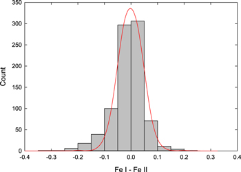
Figure 5. Histogram of Fe i – Fe ii differences for stars with an effective temperature greater than 4500 K. There are 856 stars represented in the histogram. The peak value of the Gaussian fit lies at a difference of −0.002 dex and has an FWHM of about 0.12 dex. The agreement between the Fe i and Fe ii data overall is excellent.
Download figure:
Standard image High-resolution imageAnother measure of the quality of an abundance determination is its standard deviation about the mean. The standard deviation for all species can be found in Table 6 along with the number of lines used. All errors quoted as sigma in the tables represent the line-to-line scatter only. In Figure 6, the standard deviations of the Fe i data and the number of lines utilized are presented as a function of temperature. The standard deviation of Fe i at the solar temperature (5777 K) averages about 0.04 dex with typically 500 lines used. This combination of standard deviation and number of lines means the standard error of the mean is about 0.002 dex. The behavior with temperature is as expected: the number of lines decreases away from the solar temperature, at lower temperatures due to increasing blending shifting the wavelength centroid and thus not allowing line identification. At higher temperatures, the number of lines decreases due to the overall weakening of the neutral species. The standard deviations increase toward higher and lower values for similar reasons.
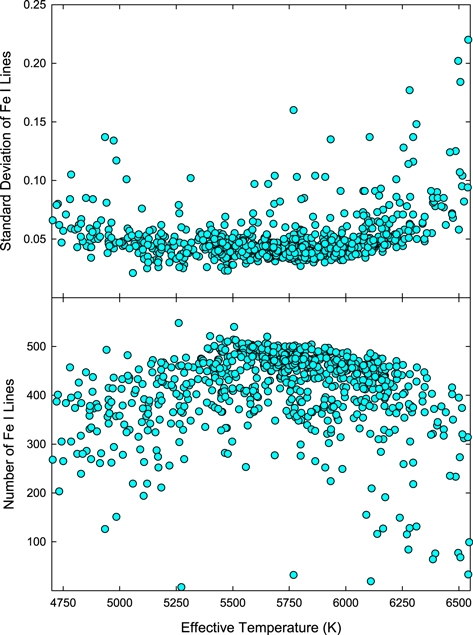
Figure 6. Top panel: the standard deviation of the Fe i abundances as a function of temperature. Bottom panel: the number of Fe i lines retained in the analysis. The standard deviation of the mean abundance at the solar temperature (5777 K) is about 0.04 dex, which when coupled to the number of lines yields a standard error of the mean of about 0.005 dex.
Download figure:
Standard image High-resolution imageA significant number of the program stars have previous analyses, and Table 7 presents iron data from a sampling of recent investigations. The offsets between the various studies are small, with the largest mean difference noted being only 0.04 dex. The agreement is excellent given the different methods of parameter determination as well as the dissimilar lines and atomic parameters used in the various analyses.
Although the comparisons in Table 7 indicate good agreement in overall scale, there can be significant differences between individual stars in parameters and iron abundance. Additionally, the differences are most often correlated. In Figure 7, the differences in temperature and gravity are shown as a function of one another. The comparison differences are this study minus the values of Suárez-Andrés et al. (2017). The Suárez-Andrés et al. values represent the most recent iteration of the Sousa et al. (2008, 2011a, 2011b) temperatures and gravities. Figure 7 shows the correlation of the gravity differences with effective temperature differences. The behavior is as expected for an excitation/ionization analysis in the sense that differences in temperature demand a corresponding gravity change to maintain equilibrium. The result is that there is little change in the derived iron abundance as one traverses the equilibrium ridge denoted by the red line in the panel. This behavior is the explanation of the agreement for the [Fe/H] ratios between the excitation/ionization studies and this work. The problem is that at temperature differences of 100 K, the gravity differences are of order ±0.22 dex. This difference means that the excitation/ionization analysis at the lower temperature will have an inferred mass assuming a constant luminosity about 0.35 solar masses lower than the masses derived here. Since the masses here are about one solar mass, the inferred mass is about 0.65 solar masses, a value that is uncomfortably low, especially at parameters near those of the Sun. The converse holds true if the temperature difference is positive.
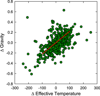
Figure 7. Variation in gravity differences as a function of difference in effective temperature. The differences shown are computed from a comparison of the results of Suárez-Andrés et al. (2017) to this work. The Suárez-Andrés et al. values represent the most recent iteration of the Sousa et al. (2008, 2011a, 2011b) temperatures and gravities. The correlation of the changes in temperature and gravity reflects the fact that in an excitation/ionization analysis, the temperature and gravity are not independent of one another.
Download figure:
Standard image High-resolution imageThe dependence of the [Fe/H] differences on temperature, gravity, and microturbulent velocity differences are more difficult to understand, as all of these differences are interrelated. A way to understand the parameter dependences of iron is given in Table 8, which shows how an iron ensemble varies with parameter changes. For the expected temperature uncertainty of ±50 K, the iron ensemble uncertainty is 0.025 for both Fe i and the [Fe/H] ratio. There is only a slight gravity dependence for these variables. These two quantities share the same parameter sensitivity as the [Fe/H] ratio is dominated by the Fe i data. The total uncertainty in the [Fe/H] ratios, line-to-line scatter, and parameter dependence is thus about 0.05 dex. The line-to-line scatter dominates this value. The error bars in all abundance figures thus indicate only the line-to-line scatter value. Note that the behavior of other species tracks that of either Fe i or Fe ii.
Table 8. Parameter Dependence of an Iron Ensemble
| Raw | Delta | [Fe/H] Delta | ||||||||||
|---|---|---|---|---|---|---|---|---|---|---|---|---|
| Temperature | Temperature | Temperature | ||||||||||
| 5708 | 5808 | 5908 | 5708 | 5808 | 5908 | 5708 | 5808 | 5908 | ||||
| Gravity | 4.16 | 7.363 | 7.429 | 7.494 | Fe i | −0.047 | 0.018 | 0.083 | [Fe/H] | −0.051 | 0.004 | 0.060 |
| 7.328 | 7.304 | 7.284 | Fe ii | −0.089 | −0.113 | −0.133 | ||||||
| 4.46 | 7.348 | 7.410 | 7.474 | Fe i | −0.063 | 0.000 | 0.063 | [Fe/H] | −0.053 | 0.000 | 0.054 | |
| 7.443 | 7.417 | 7.396 | Fe ii | 0.026 | 0.000 | −0.022 | ||||||
| 4.76 | 7.332 | 7.392 | 7.453 | Fe i | −0.078 | −0.019 | 0.042 | [Fe/H] | −0.055 | −0.005 | 0.047 | |
| 7.556 | 7.528 | 7.505 | Fe ii | 0.139 | 0.111 | 0.088 | ||||||
| Raw | Delta | |||||||||||
| Microturbulence | 0.71 | 7.474 | 0.064 | Fe i | Mean EW = 46.5 | Equilibrium | ||||||
| 7.515 | 0.097 | N = 461 | T | log g | [Fe/H] | |||||||
| 1.21 | 7.410 | 0.000 | σ = 0.043 | 5708 | 4.24 | 7.36 | ||||||
| 7.417 | 0.000 | Fe ii | Mean EW = 48.7 | 5808 | 4.46 | 7.41 | ||||||
| 1.71 | 7.348 | −0.063 | N = 55 | 5908 | 4.64 | 7.46 | ||||||
| 7.322 | −0.095 | σ = 0.066 | ||||||||||
Note. The ensemble is that of HD 59967. Raw: Fe i and Fe ii mean abundances at the temperature and gravities given. The microtubulent velocity is 1.21 km s−1. Delta: Fe i and Fe ii differences relative to the center position. The center parameters are those of Table 3. [Fe/H] Delta: Values computed thus: [Fe/H] = ((nI*AI) + (nII*AII))/(nI+nII), where "I" refers to the neutral species, "II" to the first-ionized species, n to the number of lines, and A to the abundance or [x/H] value. Columns 2, 3, and 4 in the bottom section define the microtubulent velocity response of the ensemble at T = 5808 K and log g = 4.46. Columns 7 and 8 define properties of the ensemble. The standard deviation (line-to-line scatter only) is for Table 3 parameters. Columns 11 and 12 give the equilibrium parameters and iron abundances.
Download table as: ASCIITypeset image
The possibility of temperature effects in the abundances determined here has been investigated following the finding of strong effects in L2017. Unfortunately, these abundances suffer from the same difficulties as those in L2017. In Figure 8, the abundance of Si, Ca, and Ni is shown as a function of temperature. All show an increasing abundance with decreasing effective temperature. The upward trend starts at about 5000 K and is evident by 4750 K in these three elements. This behavior echoes that of Fe ii and likely stems from the same cause, increasing blends with decreasing temperature. The silicon data also show significant scatter at near-solar temperatures. However, this is due to the presence of moderately iron-poor stars with enhanced α-elements. This effect is also present in the calcium data. Note that as in L2017, the sulfur data (not shown in a figure) have a very strong temperature effect and will therefore not be discussed further.
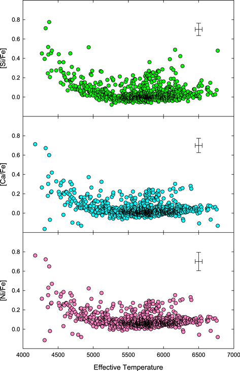
Figure 8. [x/Fe] ratios of Si, Ca, and Ni vs. effective temperature. Note the general rise in abundance below 4750 K and the increased scatter above 6500 K. The temperature related scatter is due to increasing problems with blends at lower temperatures. However, the scatter in [Si/Fe] and [Ca/Fe] at about 5750 K is real and is due to α-enhancement in metal-poor stars. The behavior with respect to temperature leads to limiting the discussion of abundances to stars in the temperature range 4750 K < Teff < 6500 K.
Download figure:
Standard image High-resolution imageIn the heavier elements, the data have been examined for temperature effects. The behavior of zirconium and barium is typical for these elements. As shown in Figure 9, there is some evidence for a temperature dependence especially in barium, but its scatter and uncertainty are larger than for the α and iron-peak elements. The most disconcerting element is neodymium. It shows a large increase in abundance as the temperature decreases, with the onset of the increase becoming apparent at 5500 K.
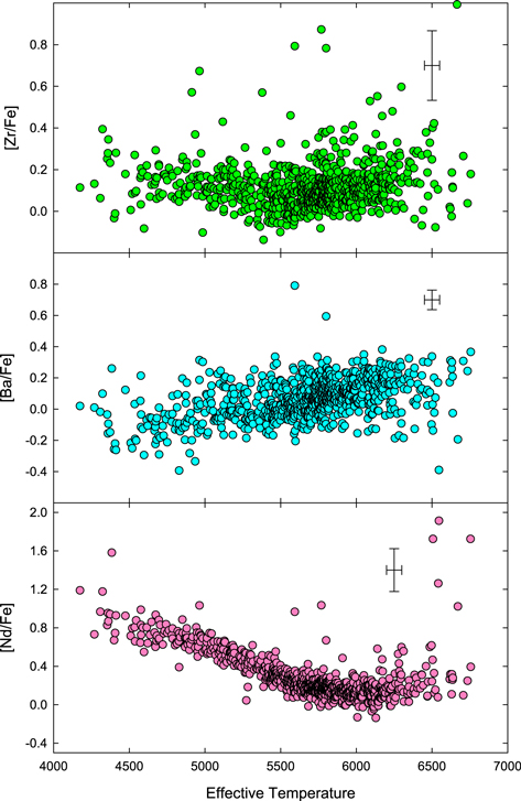
Figure 9. [x/Fe] ratios of Zr, Ba, and Nd vs. effective temperature. For Zr and Ba, there is increased scatter relative to the Fe-peak elements but little evidence for gross temperature dependences. However, for Nd, a strong temperature effect leads to placing a minimum temperature of 5500 K for consideration in the discussion. For all other elements, the effective temperature range is 4750 K < Teff < 6500 K for inclusion in the discussion.
Download figure:
Standard image High-resolution imageOnly effective temperatures above 4750 K are considered in the discussion to ameliorate the influence of the temperature trends in the data. For neodymium, the lowest temperature considered is 5500 K. It is also apparent from Figures 8 and 9 that above 6500 K there is increased scatter. Those stars have been dropped from consideration, bringing the sample size down to 806 stars.
3.2.5. Li, C, and O Abundances
In Figures 10 through 13, examples of the spectrum synthesis for C2 around 513.5 nm, the C i line at 538.03 nm, the [O i] line at 630.03 nm, and the Li feature at 670.78 nm are shown. The carbon and oxygen features are easily identified and yield good abundances. Li i shows a great range in strength as illustrated in Figure 13. At times, the line is rather strong, leading to an excellent abundance determination, but in other cases, the line is essentially undetectable, leading to an upper limit. The abundances associated with the various features are found in Table 5. For lithium, the abundance given is a limit (denoted L) if the observed depth is less than 1.5%, or in some cases, if the observed data are noisier than usual. An estimate of the non-LTE correction for lithium is also given using the data of Lind et al. (2009).
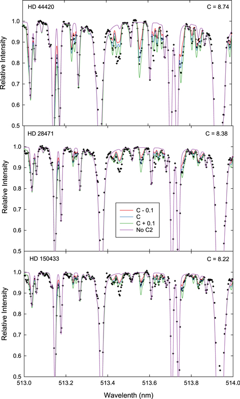
Figure 10. Syntheses of C2 near 513.5 nm for three stars all with temperatures near 5770 K but with varying carbon abundance. There are four syntheses for each star. The blue line shows the optimum fit while the red and green syntheses indicate the effect of varying the optimum abundance by ±0.1 dex. The purple synthesis has no molecular features.
Download figure:
Standard image High-resolution image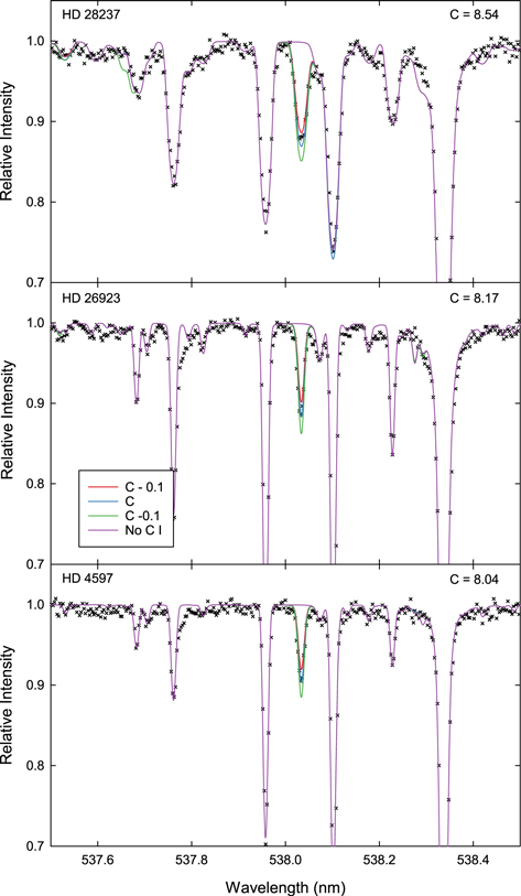
Figure 11. Syntheses of C i 538.0 nm for three stars all with temperatures near 6075 K but with varying carbon abundance. There are four syntheses for each star. The blue line shows the optimum fit while the red and green syntheses indicate the effect of varying the optimum abundance by ±0.1 dex. The purple synthesis lacks the C i line.
Download figure:
Standard image High-resolution image
Figure 12. Syntheses of the [O i] 630.0 nm line for three stars all with temperatures near 5650 K but with varying oxygen abundance. There are four syntheses for each star. The blue line shows the optimum fit while the red and green syntheses indicate the effect of varying the optimum abundance by ±0.1 dex. The purple synthesis lacks the [O i] line.
Download figure:
Standard image High-resolution image
Figure 13. Syntheses of the Li i 670.7 nm feature for three stars all with temperatures near 5860 K but with varying lithium abundance. There are four syntheses for each star. The blue line shows the optimum fit while the red and green syntheses indicate the effect of varying the optimum abundance by ±0.1 dex. The purple synthesis lacks the lithium feature.
Download figure:
Standard image High-resolution imageThe data from L2017 afford a useful comparison of lithium abundances. The parameters for this study and L2017 are very similar, so the primary difference in lithium abundances is in the quality of the data and the resulting quality of the synthesis fits. There are 76 stars in common between the two studies that have determined abundances. For these stars, the median abundance difference is +0.006 dex with a mean value of −0.002 dex. The standard deviation is 0.060 dex. Looking at the 53 stars for which at least one of the determinations is judged to be a limit, the median difference is 0.050 dex with a mean of 0.032 dex. For the stars with limits, the scatter is as expected, that is, larger with a standard deviation of 0.294 dex. The limits do not agree as well as the determined abundances as small changes in the observed profile can result in large variations in the adopted upper limit. Overall, the lithium results from the two studies agree very well.
Multiple features were used to determine both the carbon and oxygen abundances. The carbon indicators are C i 505.2 and 538.0 nm and C2. Oxygen is determined from O i 615.5 nm and [O i] 630.0 nm. The carbon data for the solar analysis indicated that the three indicators gave slightly varying answers for the carbon abundance: for C2 the derived abundance was 8.45, while C i 505.2 nm and 538.0 nm yielded 8.30 and 8.36, respectively. All three indicators were individually normalized to yield 8.43 for the solar abundance (Asplund et al. 2009), and those corrections were then applied to the final carbon abundance computation. For oxygen, the O i 615.5 nm triplet yields 8.76 for the Sun, while the [O i] 630.0 nm line yields 8.69. The latter abundance is the solar abundance adopted for this study (Asplund et al. 2009), and given that [O i] has the larger weight in the final abundance, no normalization was applied to oxygen.
To form the final carbon abundance, the features are combined as follows: (1) for T < 5250 K, only C2 is used; (2) in the range 5250 K < T < 6000 K, the simple mean of C2, C i 515.2 nm, and C i 538.0 nm is used; (3) for 6000 K < T < 6350 K, the C i lines each have weight 2, and the C2 band has weight 1; and (4) above 6350 K, the simple mean of the two C i lines is used. For oxygen, the temperature intervals are the same as for carbon, and the final average is formed as follows: (1) [O i] 630.0 nm only; (2) O i 615.8 nm has weight 1 and [O i] 630.0 nm has weight 3; (3) O i and [O i] have equal weight; and (4) O i only. These temperature regimes, especially in carbon, are the departure points for combining the features. The abundances are subject to further scrutiny, especially for temperature effects.
The possibility of systematic effects as a function of effective temperature in carbon and oxygen was examined. The C i lines used are known to show a systematic increase in abundance starting at an effective temperature of about 5000 K (Luck & Heiter 2006). The C i 538.0 nm line and the 505.2 nm line were determined in this data to be unreliable below 5500 K and 5250 K, respectively, in effective temperature.
In Figure 14, the resulting carbon abundances in the form of [C/Fe] are shown as a function of temperature. The use of [C/Fe] in this examination helps suppress variations due to overall metallicity differences between the stars. The entire temperature span of the sample is shown in the figure. It is apparent from the data that there are difficulties in the abundances. Above an effective temperature of 6500 K, the carbon abundances rapidly become highly scattered. The scatter is due to the prevalence of significant total broadening velocities at these temperatures, and thus, an inability to adequately model the C i line profiles. This effect was seen in other abundances. Below an effective temperature of about 5000 K, there is an uptick in the [C/Fe] ratios. The [C/Fe] ratio does vary with overall metallicity, but the scatter seen here is larger than what one would expect, and there is a general trend toward higher carbon content with decreasing temperature. Carbon abundances below 5250 K depend solely on C2; therefore, the problem is likely the increasing contamination of the C2 lines by other atomic and molecular species with decreasing temperature. In further discussions of the carbon abundances, only abundances from stars in the effective temperature range 5000–6500 K will be considered.

Figure 14. [C/Fe] vs. effective temperature for the entire sample of dwarfs. Note the discrepant [C/Fe] ratios above 6500 K and the uptick in [C/Fe] below 5000 K. The most likely explanation for the uptick below 5000 K is intruding unaccounted for blends in the C2 lines and difficulty with total broadening in the hotter stars.
Download figure:
Standard image High-resolution imageThe differences in abundance estimates between the various carbon indicators show that they yield consistent answers after the normalization to the solar abundance. The mean difference between the two C i lines is −0.001 dex (505.2–538.0), and the difference between those two lines and the C2 feature averages −0.05 and −0.03 dex, respectively. The standard deviation about the mean is about 0.0.6–0.09 dex. For the two oxygen indicators, the O i triplet averages +0.06 dex relative to the [O i] line. The standard deviation for this comparison is about 0.1 dex. Note that no trends in the oxygen indicators are present in the data in the temperature range to be considered in the overall discussion of abundances, that is, 4750–6500 K.
In Table 7, the mean differences in the carbon and oxygen abundances determined here and in several recent analyses are presented. Figure 15 shows the comparison of the results found here versus those in Suárez-Andrés et al. (2017) for carbon. Basic statistics for the comparison are found in Table 7. The mean difference in [C/H] is +0.02 dex (this work larger). The difficulty in the comparison is the scatter below the main locus of the data—see Figure 15. The scatter partially results from residual effects that taint C2 below 5000 K in this study. Another difficulty is that the [C/H] differences correlate with the temperature and gravity differences, with carbon differences of +0.4 dex (this study larger) usually being associated with gravity differences of about +0.2 dex.
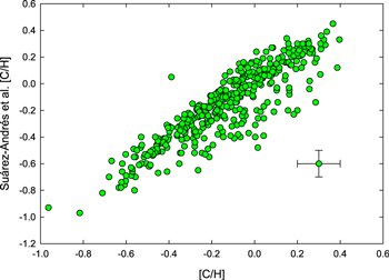
Figure 15. [C/H] data of Suárez-Andrés et al. (2017) vs. the [C/H] ratios of this study. A few more metal-poor stars have been excluded from the plot to facilitate examination of the bulk of the data. Overall, the comparison is good. The scatter below the mean locus is discussed in Section 3.2.5.
Download figure:
Standard image High-resolution imageThe features used to determine oxygen abundances in dwarfs, the O i line at 615.5 nm, and the [O i] line at 630.0 nm are rather weak. Typical equivalent widths for these lines are 0.005–0.010 nm. Figure 12 shows syntheses of the [O i] line and its surrounding area. Although weak, the line is usable. Bertran de Lis et al. (2015) determined oxygen abundances in many of these dwarfs using the same oxygen lines. Figure 16 shows the comparison of the [O/H] ratios. The scatter is as expected given the strength of the lines involved, and the systematics are good; the mean difference is 0.01—see Table 7.

Figure 16. [O/H] data of Bertran de Lis et al. (2015) vs. the [O/H] ratios of this study. Given the difficulty in determining the oxygen content from the weak O i 615.5 nm and [O i] 630.0 nm features, the comparison is acceptable. The solid red line is the line of equality.
Download figure:
Standard image High-resolution imageIn returning to the overall data presented for carbon and oxygen in Table 7, one finds that the systematic agreement is excellent, with the mean differences in all cases 0.05 dex or less. The spread in abundances as typified by the standard deviation is generally of order 0.1 dex and is as expected based on the different methods and the general weakness of the oxygen abundance indicators especially. A handful of stars are in common between this study and the non-LTE analysis of Zhao et al. (2016). These stars are among the most metal poor in this study and likely show the most pronounced NLTE effects. At near-solar temperatures and metallicity, the Zhao et al. NLTE abundances are generally within 0.1 of the LTE values for all species.
4. Discussion
In the past several years, there have been several extensive discussions of abundances in the local neighborhood and their relation to galactic chemical evolution (Nomoto et al. 2013; Hinkel et al. 2014; Brewer et al. 2016). Bensby et al. (2014) discussed local abundances and kinematics. Here, only the most salient features of the local abundances are considered.
4.1. Z > 10 Abundances
Among the Z > 10 elements, there are well-documented trends. These include the decrease in the [x/Fe] ratios with increasing [Fe/H] among the α-elements and the increase in the [Mn/Fe] ratio with increasing [Fe/H]. In Figure 17, the α-elements silicon and calcium exhibit the expected behavior. The α-elements come from two sites, Type II and Type Ia supernovae (Johnson 2017), and the dependence of their [x/Fe] ratios reflects the growing importance of SNe Ia element production as a function of time. Manganese is produced predominately in SNe Ia (Kobayashi & Nomoto 2009). The increase in [Mn/Fe] with increasing [Fe/H] thus reflects the increased production of manganese with time.

Figure 17. [Si/Fe], [Ca/Fe], [Mn/Fe], and [Ni/Fe] vs. [Fe/H]. The trends seen in silicon and calcium reflect the increasing importance of SNe Ia relative to SN II as a function of time. The trend in manganese reflects its origin in SNe Ia. The error bars shown are the means of the individual standard deviations per element taken across the sample. A more extended discussion is given in Section 4.1.
Download figure:
Standard image High-resolution imageAlso shown in Figure 17 is the behavior of [Ni/Fe] as a function of [Fe/H]. Since nickel is the precursor element for iron nucleosynthesis, the tight and nearly flat relation up to [Fe/H] about −0.1 is no surprise. What is seen in Figure 17 (bottom panel) starting at [Fe/H] ∼ 0 is an upturn in the [Ni/Fe] ratio. The [Ni/Fe] ratio increases from about 0 at [Fe/H] about 0 to a ratio of +0.1 at [Fe/H] of +0.4. What is interesting is that the same behavior is present in the [Mn/Fe] data. This similarity was noted by Luck (2015, 2017).
The behavior of a sample of the s- and r-process elements with Z > 38 are shown in Figure 18. The elements zirconium and barium (top two panels) show very similar behavior vis-à-vis [Fe/H]. Both have essentially [x/Fe] = 0 up to [Fe/H] about 0 where both tail off toward lower [x/Fe] ratios. The effect in barium is more obvious than what is seen in zirconium. Both are predominantly s-process elements formed in post-AGB stars (Johnson 2017), but zirconium has a contribution from SNe II, while barium has a contribution from the r-process elements ostensibly from merging neutron stars (Johnson 2017; Pian et al. 2017; Tanvir et al. 2017). From their similar behavior, it appears that the post-AGB component dominates the abundance.

Figure 18. [Zr/Fe], [Ba/Fe], [Nd/Fe], and [Eu/Fe] vs. [Fe/H]. Note the differing behavior of the almost pure s-process element barium and the r-process element europium. The error bars shown are the means of the individual standard deviations per element taken across the sample. The lack of abundance error bar for europium reflects the fact that the abundance is determined from a single line. A more extended discussion is given in Section 4.1.
Download figure:
Standard image High-resolution imageThe next element down in Figure 18 is neodymium. It has almost equal contributions from the s- and r-processes (Johnson 2017), and the abundances do not show any discernible trend with [Fe/H]. The bottom panel of Figure 18 shows the behavior of the almost pure r-process element europium. It shows a decrease in the [Eu/Fe] ratio with increasing [Fe/H] with perhaps a flattening of [Eu/Fe] above [Fe/H] ∼ 0. This behavior has been noted in other studies, including Brewer et al. (2016).
A common way to examine abundances is to examine the systematics of the [x/Fe] ratios as a function of atomic number. In Figure 19, this information is displayed. The mean ratios of [x/Fe] shown in Figure 19 are limited to −0.2 < [Fe/H] < +0.2 in order to try to mitigate the influence of trends in [x/Fe] ratios on [Fe/H]. It is evident that most elements show an [x/Fe] ratio near 0. The exceptions are the heavier s-/r-process elements that show a modest enhancement over the solar values. This enhancement was also noted by Luck (2017). The question posed there is still pertinent: are the stars of the local region overabundant in these elements, or is the Sun underabundant?
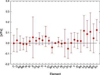
Figure 19. [x/Fe] ratios vs. element. The stars used to determine the raw ![$\langle [{\rm{x}}/\mathrm{Fe}]\rangle $](https://content.cld.iop.org/journals/1538-3881/155/3/111/revision1/ajaaa9b5ieqn19.gif) ratios are limited to −0.2 < [Fe/H] < +0.2. Note that these stars have iron-peak ratios consistent with solar values, but that the heavy r-process elements are more abundant than those found in the Sun.
ratios are limited to −0.2 < [Fe/H] < +0.2. Note that these stars have iron-peak ratios consistent with solar values, but that the heavy r-process elements are more abundant than those found in the Sun.
Download figure:
Standard image High-resolution image4.2. Li and [Fe/H] in Dwarfs
Lithium in dwarfs is a subject of some controversy, especially in the comparison abundances of planet-host stars to stars not known to host a planet: see, for example, the conclusions of Gonzalez (2014, 2015) versus those of Luck (2017). This sample includes 128 hosts, the planets of some of which are close giant planets (Exoplanets team 2017). The lithium abundances as a function of temperature and mass are shown in Figure 20. As can be readily seen, the abundances show a strong dependence on temperature and mass, with a substantial decline in abundance setting in between 5800 and 6000 K. This decline is not a new finding. It was noted by Lambert & Reddy (2004) and subsequently by Luck & Heiter (2007) as well as by Luck (2017). The astration of lithium as a function of temperature is due to the increasing convection depth with decreasing mass. The stellar mass at the onset point of strong lithium astration is in the range of 0.8–1.0 solar masses.
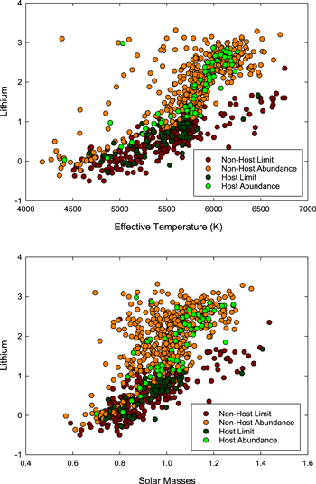
Figure 20. Abundance of lithium vs. effective temperature (top panel) and mass (bottom panel). The effect of temperature- (mass-) dependent astration of lithium is evident, setting in a most pronounced fashion at about 5800 K, corresponding to about 1 solar mass. The data are separated between determined abundances, upper limits, and planet host vs. non-host.
Download figure:
Standard image High-resolution imageIn Figure 20, the host stars are designated differently from the non-host stars, but they are difficult to pick out in the corpus of data. To better discriminate between the hosts and the non-host, a box-whisker plot of the data is shown in Figure 21. The bin size of the plot is 200 K, and only stars with determined abundances are considered. The box limits are at the 25th and 75th percentile levels in abundance, with the whiskers at the 10th and 90th percentile level. Indicated in the boxes are both the mean and mode of the abundances. This plot indicates that for temperatures above 5800 K, there is no significant difference between the lithium abundances, and that in the temperature range 5400–5800 K, the non-host lithium abundances are larger than the hosts'.
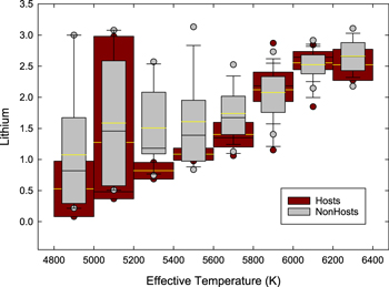
Figure 21. Box and whisker plot comparing the host (red boxes) and non-host (gray boxes) lithium abundances as a function of temperature. Each bin is 200 K wide. The box heights are limited by the 25th and 75th percentile levels while the whiskers indicate the 10th and 90th percentile levels. The outermost circles indicate the 5th and 95th percentiles. Within each box, the median is the black line, and the mean is the yellow line. This display information is common to all box plots of this paper. There is no discernible difference between the hosts and non-hosts in lithium abundances.
Download figure:
Standard image High-resolution imageLithium abundances in dwarfs are known to correlate with age (Carlos et al. 2016 and references therein). Lithium abundances also show a mass–metallicity correlation (Lambert & Reddy 2004. However, the situation with planet hosts is not that clear concerning age, as Delgado Mena et al. (2014, 2015) argue that planet hosts have lower lithium abundances than non-host stars and thus age is not the only factor contributing to differences in lithium abundances. Note that the conclusion reached here does not support that inference. Although ages were determined for this sample, they are insufficiently reliable to contribute to this facet of lithium abundances in dwarfs. What is possible for this sample is to examine the lithium content versus planet mass. If one plots the determined lithium abundances versus the maximum-mass planet in a system, one obtains a correlation in the sense that systems with lower maximum-mass planets have lower lithium abundances. However, the meaning of this relation is not clear as those abundances correlate strongly with the temperature of the host star.
The overall metallicity of host versus non-hosts stars has been examined in previous works (Gonzalez 1997; Fischer & Valenti 2005; Luck & Heiter 2006; Buchhave et al. 2012; Luck 2017). The overall result is that [Fe/H] ratios in systems with high-mass planets orbiting close to their parent star, i.e., hot Jupiters, have higher [Fe/H] ratios on average compared to systems either with lower-mass planets or massive planets several astronomical units from the host, or non-host stars. In Figure 22, the [Fe/H] ratios of the host stars are shown versus the maximum-mass planet known in the system. The data are divided into three categories: (1) hosts that have a planet of mass greater than 0.8 MJupiter within a semimajor orbital radius of 0.5 au of the host, (2) systems that have a planet of 0.2 MJupiter within a semimajor orbital radius of 1.0 au of the host, and (3) lastly, the remaining systems. The general behavior is that the [Fe/H] ratios increase from about −0.4 at planet mass 0.003 MJupiter to near solar at 0.1 MJupiter. At that point in planet mass, the sub-Jupiters and hot Jupiters start to dominate the systems and have [Fe/H] ratios above solar. Although above-solar [Fe/H] ratios are frequent in systems with more massive planets, there are exceptions, with HD 134113 being a prime example.
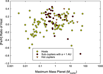
Figure 22. [Fe/H] ratios of the planet hosts vs. the maximum mass of the known planets in the system. The data are segregated according to whether there is a "hot Jupiter" in the system, a sub-Jupiter within one astronomical unit of the host, and the remaining hosts. The [Fe/H] content reaches a plateau at about 0.1 MJupiter. Some scatter to lower abundances at higher planetary mass is evident.
Download figure:
Standard image High-resolution imageA caveat concerning the above discussion relates to the idea of planets of known mass. Detection biases operate against high-mass planets at large distances from their host. Additionally, it is difficult to detect lower-mass planets in "close" orbits around active, young, and presumably more metal-rich hosts. The detection of such systems could fill in the underpopulated regions of Figure 22.
As a last point about hosts versus non-hosts, a histogram of [Fe/H] values for the two sets is shown in Figure 23. As demonstrated above, the hosts show a preference for higher [Fe/H] values. In this data, the peak values of the two distributions are separated by 0.09 dex. This difference is somewhat smaller than the value of 0.12 dex found by Luck (2017) but is not significantly dissimilar.
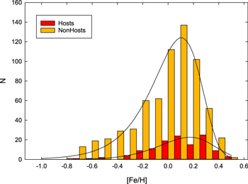
Figure 23. Distribution of [Fe/H] ratios for hosts vs. non-hosts. The smooth fits are the four-parameter Weibull distributions whose maximums differ by 0.067 dex. Note the presence of several moderately metal-poor stars among the hosts.
Download figure:
Standard image High-resolution image4.3. C and O in Dwarfs
Carbon and oxygen abundances in dwarfs display the sum of galactic chemical evolution appropriate to their time and place of formation. The trends for both are decreasing [x/Fe] ratios with increasing [Fe/H]. This expectation is borne out for both as seen in Figure 24. Both [C/Fe] and [O/Fe] decrease with time due to the increasing importance of SNe Ia fueling the increase in iron. However, the slopes of the two relations are different, giving rise to the variation in the C/O ratio as a function of [Fe/H] seen in the bottom panel of Figure 24. This dissimilarity is due to differing yields for carbon and oxygen because of their different sites of production. Carbon is the direct result of He burning, with oxygen being a common follow-on product to He burning, but the oxygen production site for chemical enrichment is SNe II, while carbon is created in lower-mass post-AGB stars shedding mass to end their life as white dwarfs (Johnson 2017).

Figure 24. [C/Fe], [O/Fe], and C/O vs. [Fe/H]. The trends seen here are well known. The decrease in [O/Fe] with increasing [Fe/H] reflects the increasing importance of SNe Ia with time relative to SNe II. Carbon is a product of post-AGB stars with masses insufficient to undergo SNe II detonations. The different origins of these two elements are reflected in the behavior of the C/O ratio. Several stars with [Fe/H] < −1 are not shown.
Download figure:
Standard image High-resolution imageExamining the C/O ratios found in these dwarfs, the mean C/O ratio for stars within ±0.2 dex of [Fe/H] = 0 is +0.51, which compares very well with the solar C/O ratio of 0.55.
Dwarfs in the mass range of this study are the progenitors of normal G and K giants. Standard evolutionary models for 0.7–3 solar masses (Iben 1967) indicate that giants that have undergone the first dredge-up should be carbon diluted and show no difference in oxygen abundance relative to their original composition. In Figure 25, a box and whisker plot of the carbon and oxygen abundances of this study are shown versus the carbon and oxygen abundances from the giant study of Luck (2015). More specifically, Figure 25 shows [x/Fe] versus [Fe/H] binned at 0.2 dex in [Fe/H]. As expected, the giant carbon content is lower than the dwarf content, and there is no difference in the oxygen abundances. Gratifyingly, on the whole, standard stellar evolution works.

Figure 25. Box and whisker plot of [C/Fe] and [O/Fe] vs. [Fe/H] showing both the dwarfs of this study and the giants of Luck (2015). The carbon abundances of the giants are offset from the dwarf abundances and reflect the changes predicted by standard stellar evolution. Standard stellar evolution predicts no changes to the surface oxygen content during the evolution to a giant. The observed data support this conclusion.
Download figure:
Standard image High-resolution image
5. Concluding Remarks
This study analyzed a sample of nearby dwarfs in the hope of establishing the standard of normalcy in the local region around the Sun. The results are that the Sun is very akin to the stars of the local region. If the [Fe/H] ratio of a local dwarf is within ±0.2 of the Sun, its abundances, overall, are solar. There are two possible exceptions:
- 1.The abundance of lithium can be anywhere from log εLi = 1 to 3—a range of two orders of magnitude.
- 2.The lanthanides with Z = 57 are somewhat enhanced relative to the Sun.
Regarding future studies of this type, the most pressing need is to extend the temperature range reliably down to at least early M-type stars around 3500 K. This will not be possible in the optical due to strong blending and line strength problems but should be possible in the near-infrared. However, lack of atomic and molecular data will be a major problem.
The comments and questions of an anonymous referee led to manifest improvements in this paper. The SIMBAD database, operated at CDS, Strasbourg, France, and satellite sites, and NASA's Astrophysics Data System Bibliographic Services were instrumental in this work. The HARPS spectra were acquired through the ESO Data Archive Portal. The data are drawn from 145 different programs with program 072.C-0488(E) contributing over 300 spectra.