


Abstract
We present optical V band albedo distributions for middle solar system minor bodies including Centaurs, Jovian Trojans, and Hildas. Diameters come mostly from the NEOWISE catalog. Optical photometry (H values) for about two-thirds of the ∼2700 objects studied are from Pan-STARRS, supplemented by H values from JPL Horizons (corrected to the Pan-STARRS photometric system). Optical data for Centaurs are from our previously published work. The albedos presented here should be superior to previous work because of the use of the Pan-STARRS optical data, which is a homogeneous data set that has been transformed to standard V magnitudes. We compare the albedo distributions of pairs of samples using the nonparametric Wilcoxon test. We strengthen our previous findings that gray Centaurs have lower albedos than red Centaurs. The gray Centaurs have albedos that are not significantly different from those of the Trojans, suggesting a common origin for Trojans and gray Centaurs. The Trojan L4 and L5 clouds have median albedos that differ by ∼10% at a very high level of statistical significance, but the modes of their albedo distributions differ by only ∼1%. We suggest the presence of a common "true background" in the two clouds, with an additional more reflective component in the L4 cloud. We find, in agreement with Grav et al. that the Hildas are darker than the Trojans by 15%–25%. Perhaps the Hildas are darker because of their passage near perihelion through zone III of the main asteroid belt, which might result in significant darkening by gardening.
Export citation and abstract BibTeX RIS
1. Introduction
Minor solar system objects in the vast "middle kingdom" of the solar system, from roughly the main asteroid belt to the classical Kuiper Belt, may hold key clues to the history of the solar system, particularly in regards to the idea that planetary migration was a major sculptor of the solar system. In the middle kingdom, we find the Hildas and Jovian Trojans, objects in low order orbital resonances with Jupiter, and the Centaurs, objects on dynamically unstable orbits crossing the orbits of the outer planets. The Hilda and Trojan populations each contain a few currently identified dynamical families of objects. As the objects in each family presumably share a common origin and similar history, comparison of the properties of family objects with the general background in which they are found may give clues as to how surface composition and surface history affect observable physical properties such as color and albedo (A). Comparison of the physical properties of these different populations of objects, as well as comparison of families in each population, should lead to a better understanding of the relationships between the classes and their histories.
In this paper, we utilize new infrared and optical surveys of large samples of middle kingdom objects to compare one physical property- the V band albedo- between various samples of objects. The albedo or reflectivity of minor solar system bodies is related to their surface chemical composition and surface processing history. Of course the albedo is not a unique signature of surface composition or history, as different scenarios can yield the same albedo. Nevertheless, as it is becoming possible to determine reasonably accurate albedos for large numbers of objects, study of albedos for different populations of objects might help suggest connections between populations and/or help disentangle the effects of differing surface histories.
Determination of albedo requires both a size measurement and a measurement of the optical brightness of a body. The optical brightness is usually specified by the H magnitude. As for sizes, a few objects can be observed by stellar occulations to determine sizes, and sizes can also be determined for objects in some binary systems. However, the vast majority of sizes for middle kingdom objects come from observations of their thermal emission.
Diameters for thousands of Hildas and Trojans and dozens of Centaurs have become available from observations performed by the NEOWISE component of the Wide-field Infrared Survey Explorer (WISE; Wright et al. 2010, Mainzer et al. 2011). Photometrically calibrated optical H magnitudes are becoming available for hundreds of thousands of minor bodies as the result of large sky surveys. In this paper, we use the NEOWISE diameters, supplemented by diameters for Centaurs from Spitzer Space Telescope and Herschel, coupled with the H magnitudes from the Pan-STARRS PS1 survey (Veres et al. 2015), JPL Horizons, and our Centaur photometric survey to determine albedos for several thousand middle kingdom objects. We then compare the albedo distributions of the various samples of objects using the nonparametric Wilcoxon rank sum test.
2. IR and Optical Data
Because of the ongoing effort of the Minor Planet Center to assign minor planet numbers, object lists that contain objects with only provisional designations can become outdated as objects are numbered, which can complicate matching different lists. To ensure accurate and complete matching between lists, all lists were updated to designations current as of 2016 September 1. Thus, each object has a unique designation in all of our lists, either a number or a packed provisional designation.
All diameters of Trojans and Hildas come from the NEOWISE catalog found at the NASA Planetary Data System (Mainzer et al. 2016). The Jupiter Trojan table has 1860 entries. These represent 1858 distinct objects, as two objects were listed twice, with different diameters. For these two objects, a weighted average diameter was calculated. The 1858 objects were matched with the list of Jovian Trojans at the Minor Planet Center,4 as updated on 2016 August 20. Eight objects in the NEOWISE catalog were not found in the Trojan list. These objects were found to have very short astrometric arcs or had been found to be non-Trojans. Of the remaining 1850 NEOWISE Trojans, 1075 were in the L4 (leading) cloud and 775 in the L5 (trailing) cloud. As of 2016 September 1, 97.3% of these Trojans had been assigned minor planet numbers.
In statistical investigations such as this, one must always be on the lookout for biases in the sample, particularly for objects near the limit of detection. Grav et al. (2011) say the Jovian Trojans are complete to a diameter limit of 10 km. We eliminated from the sample the 77 objects (4.2%) with listed diameters of less than 10 km.
We found all Trojans in the (3548) Eurybates dynamical family in the L4 cloud, using the family list for Trojans and Hildas5 (Broz & Vokrouhlicky 2008). Of the 171 objects in the Broz and Vokrouhlicky list, 75 were in the NEOWISE D > 10 km list. Of the 34 objects in the (4709) Ennomos family list, 14 were in the NEOWISE D > 10 km list. The objects in the (3548) Eurybates family list were removed from the NEOWISE L4 list to give a sample we call the "L4 background", although of course this "background" sample may well contain additional families not yet recognized. We did the same for the L5 list and the (4709) Ennomos family.
The Hilda NEOWISE catalog contains 1090 entries, with 66 objects having two entries, leaving 1024 unique objects. For the Hildas, Broz and Vokrouhlicky list members of two dynamical families, associated with (153) Hilda and (1911) Schubart and we separated these from the background Hilda population. The (153) Hilda dynamical family contains 215 NEOWISE objects with D > 5 km and the (1911) Schubart family has 111 NEOWISE D > 5 km objects. The background Hilda population, with the (153) Hilda and the (1911) Schubart families removed, contains 555 D > 5 km NEOWISE objects.
Some may question the accuracy of diameters derived from single band NEOWISE detections, given that there may be some dependence on HV for diameter determinations for single band detections and that the NEOWISE HV are slightly different from the ones we use. We do not think this is a major concern. Only a small fraction of objects have only a single band detection: about 7% of Trojans and 13% of Hildas. We looked at the derived albedos for single versus multiple band detections to look for any systematic difference. For the four largest samples, where there are enough single band detections to get a good statistical comparison with multiband detections in the same sample (Trojan L4 and L5 backgrounds, Hilda background and Hilda (153) family), we compared the median albedos of the single versus the multiband detected objects within each sample using the Wilcoxon test. For the four samples, p-values range from 0.3 to 0.8, indicating no significant difference between the medians of the albedo distributions of single and multiband detections. We also computed the standard deviations of the distributions of the logarithms of the albedos for single and multiple band detections within each sample. (As discussed below, the sample albedo distributions are approximately lognormal.) The single band detections have a slightly larger standard deviation in albedo (average of the four sample standard deviations in logarithm for single band detections is 0.18 versus 0.15 for multiband detections). This slight increase in albedo scatter for the single band detections is not surprising, as the single band detected objects tend to be fainter than the multiband detected objects.
Determination of optical albedo requires a measurement of the optical brightness of the object. This is commonly expressed as the absolute magnitude, H, the V magnitude that the object would have if observed at 1 au from both Sun and Earth at a phase angle of zero. For asteroids, accurate H values require photometrically calibrated observations over a complete rotational period of each asteroid near solar opposition. Observations made away from opposition require assumption of a solar phase curve, the relationship between magnitude and solar phase angle. Because of the time required to obtain such observations, particularly for objects with rotational periods longer than a typical night, only a very small fraction of asteroids have H values of the quality that is obtainable with present methods. The NEOWISE infrared observations are made so that each minor planet receives on average 10−12 observations over a ∼36 hr period (Wright et al. 2010; Mainzer et al. 2011). Thus, the typical object has a reasonably complete rotational averaging in the infrared.
At present, the only database with H values for virtually every asteroid is the JPL/MPC. These H values are largely derived from observations taken for astrometric purposes by a variety of telescopes. Thus these magnitudes are not usually optimized for photometric accuracy, as discussed in detail in Veres et al. (2015). However, new surveys are becoming available that contain more accurate H estimates for large numbers of asteroids. One such survey, which give H values for almost 250,000 asteroids, has been published by Veres et al. (2015). The available version v1.0 catalog6 is based on observations from 2011 February until 2012 May using the Pan-STARRS PS1 telescope. The observations were made in six Sloan-like filters, but the H values have been transformed into the standard V system. The catalog gives several estimates of H, based either on the Bowell et al. (1989) or the Muinonen et al. (2010) formalism for phase angle correction. As the objects of concern here typically have only a handful of actual observations each in the Pan-STARRS catalog (median number of observations is 4), we do not see any reason to prefer one or the other H magnitude. For all the Hildas and Trojans in both the NEOWISE and Pan-STARRS catalogs, we find a mean difference between the Bowell H mag (HB; not to be confused with H in the B filter) and the Muinonen H mag (HM) of only 0.03 mag. We simply use an average of HB and HM, which we designate as HPS, for Pan-STARRS H.
Of the 1773 D > 10 km Trojans, 1341 (76%) have an entry in the Pan-STARRS database. Of the 881 D > 5 km Hildas, 606 (69%) have an entry. Thus, while the majority of Hildas and Trojans in the diameter limited samples have HPS values, a sizable fraction do not. Many of the objects not in the Pan-STARRS catalog are undoubtedly fainter objects, but others are presumably missing due to the limited time frame of the v1.0 catalog. To avoid possible bias due to non-inclusion of optically faint objects, we turn to the H values from JPL Horizons7 to estimate an H value for objects that are in the NEOWISE database but not in the Pan-STARRS database, so that we have an H value for every object that has a NEOWISE diameter. First, we must compare the JPL H values with the Pan-STARRS values and derive a way to determine H values on the Pan-STARRS system for objects with only a JPL H values available.
In Romanishin & Tegler (2005), we found that the JPL H values were on average too bright by 0.34 mag for a sample of KBOs and Centaurs for which there was good V band photometry. For the present samples, we first worked with H values listed in the NEOWISE catalog, which we refer to as HNEO. The HNEO values are from JPL Horizons at the time the NEOWISE catalog was compiled. We found the difference HNEO − HPS for all the Hildas and Trojans with HPS values, regardless of diameter (2014 objects). The differences, plotted against HNEO, are shown in panel (a) of Figure 1. For objects fainter than H of 11, the mean (and also median) difference HNEO − HPS is −0.35, with a standard deviation of 0.29. These values are remarkably similar to what we found in Romanishin & Tegler (2005). The difference is less for objects brighter than H = 11. We suspect brighter objects have more accurate H values available that have been incorporated into the JPL database used in the NEOWISE catalog.
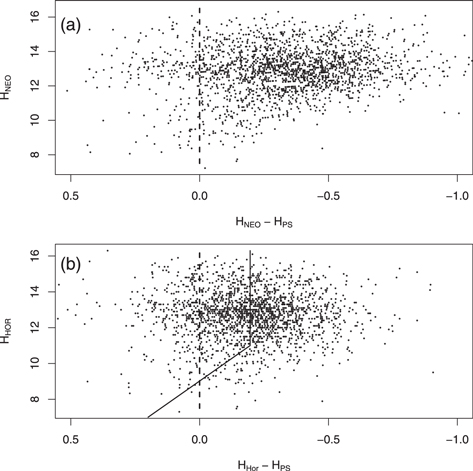
Figure 1. (a) The difference HNEO − HPS vs. HNEOfor 2014 Hildas and Trojans. (b) The difference HHor − HPS for the same sample. The solid dark line is the relationship used to correct HHor to HPS. To the right of each dashed vertical line, the JPL H value (HNEO or HHor) is too bright. The top panel shows that the HNEO values, the H values found in the NEOWISE database, are too bright on average by 0.35 mag. The bottom panel shows that the more recent (as of 2016 November) H values from HORIZONS (HHor) are closer to the HPS values, but are still too bright on average by 0.20 mag.
Download figure:
Standard image High-resolution imageHowever, we noticed that the current JPL Horizons database contains H values that have been updated since the NEOWISE catalog was compiled and so differ from HNEO values. We found current (as of 2016 November) H values from Horizons for all our objects in the NEOWISE catalog. We refer to these more recent Horizons H values as HHor. Panel (b) of Figure 1 shows the difference between HHor and HPS for the same 2014 objects. Comparison of HHor and HPS for the objects fainter than H = 11 shows a mean difference of −0.20, with a standard deviation of 0.23. Thus the HHor values are definitely closer to the HPS values than are the HNEO values. We conjecture that the remaining systematic offset is due to a passband effect, as the JPL values would make more sense if they referred to a passband somewhat to the red of V, say a V + R, and present evidence for this below.
As the Pan-STARRS values have been transformed to the standard V photometric system, we want to transform the HHor values to the Pan-STARRS system. We derived a simple transformation between HHor and HPS as shown in the lower panel of Figure 1. This is a simple offset for objects fainter than H = 11 and a simple linear relation for the brighter objects. Only a few percent of the objects that did not have Pan-STARRS photometry were brighter than H = 11, so for the vast majority of the objects without Pan-STARRS photometry only the offset was needed to transform from HHor to HPS.
In Tegler et al. (2016), optical colors and H are presented for a sample of 62 Centaurs. These H values, which we will call HTRC, were all taken under photometric conditions and are on the standard V system. We compared the HTRC values with the HHor values for the Centaurs. Figure 2 shows the difference in H values versus the color index B − R. The median HHor − HTRC is −0.16 for the gray Centaurs and −0.49 for the red Centaurs. A Wilcoxon test shows the gray and red H sample differences differ significantly (p = 0.0001). The red objects have systematically brighter H values, suggesting that the HHor values might refer to a redder effective wavelength than the V passband. Note that the HHor − HPS difference for the gray Centaurs (−0.16) is similar to that for the Trojans and Hildas (−0.20). We note that the Trojans have B − R colors similar to the gray Centaurs (Tegler et al. 2008). We have V − R colors for the Centaurs, so we can estimate H values at wavelengths redder than V. As shown panel (b) in Figure 2, for H at a wavelength about midway between V and R the average of the gray and red HHor − HTRC is about zero. There is still a difference between the gray and red Centaurs, but the difference in reduced. As many astrometric observations use CCDs with broad filters or even no filter, there is probably a substantial color term in the relation between true H and HHor, even if we are correct in our conjecture that HHor refers to a passband with a central wavelength roughly between V and R.
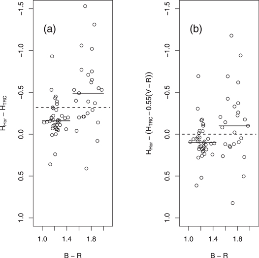
Figure 2. (a) The difference between HHor and HTRC is plotted vs. B − R for the 62 Centaurs in Tegler et al. (2016). The solid horizontal line segments mark the median values for the gray and red samples. The horizontal dashed line is the average of the gray and red medians. (b) The difference between HHor and the H value with a passband that is approximately V + R, as discussed in the text. The solid and dashed lines are the same as in (a). The left panel shows that the HHor values for the gray Centaurs are too bright by 0.16 mag and the HHor values for the red Centaurs are too bright by 0.49 mag. The right panel shows that the difference between HHor and HTRC for Centaurs can be eliminated if we assume the HHor value refers to a bandpass to the red of V.
Download figure:
Standard image High-resolution imageHow bright are the sample Trojans and Hildas in the optical? For all of the Trojan asteroids larger than 10 km that have a value of HPS, the median HPS is 12.7. For all of the Hildas larger than 5 km with available HPS, the median value is 14.23. At its average solar distance, when at opposition the median Trojan would have an apparent V mag of 19.4 and the median Hilda 19.6. Of course, the objects would be systematically fainter than this due to observation away from opposition. Also, of course, the actual heliocentric distances vary due to eccentricty of the orbits, particularly among the Hildas, which have an average orbital eccentricity of approximately 0.2, significantly larger than the Trojans, which have a typical eccentricity of 0.05.
Basic information on the nine samples considered are presented in Table 1. Columns 2 and 3 give the sample size and median albedo for the "mixed H" samples that use HPS if available and transformed HHor values otherwise. Columns 4 and 5 give sample size and median albedo for samples using only Pan-STARRS photometry, or in the case of the Centaurs, only photometry from Tegler et al. (2016). The last column gives a short name used in Table 2. There are no mixed H samples for the Centaurs, as we used only objects for which we have photometry (H values and colors).
Table 1. Number of Objects and Median Albedos of Samples
| Sample | Mixed H | PS/TRC H Only | Short Name | ||
|---|---|---|---|---|---|
| N | Median A | N | Median A | (for Table 2) | |
| L4 background | 944 | 0.0554 | 762 | 0.0581 | L4 |
| L5 background | 740 | 0.0505 | 519 | 0.0517 | L5 |
| (3548) Eurybates family | 75 | 0.0466 | 53 | 0.0492 | Eur |
| (4709) Ennomos family | 14 | 0.0494 | 7 | 0.0473 | Enn |
| Hilda background | 559 | 0.0437 | 378 | 0.0457 | Hbac |
| (153) Hilda family | 216 | 0.0443 | 160 | 0.0440 | Hfam |
| (1911) Schubart family | 111 | 0.0309 | 72 | 0.0310 | Sch |
| Gray Centaurs | ⋯ | ⋯ | 25 | 0.0500 | GraC |
| Red Centaurs | ⋯ | ⋯ | 11 | 0.1120 | RedC |
Download table as: ASCIITypeset image
Table 2. Pairwise P-values
| Pair | Mixed H | PS/TRC H Only | ||||
|---|---|---|---|---|---|---|
| p-value | ΔA | ΔA 95% range | p-value | ΔA | ΔA 95% Range | |
| L4–L5 | 4.0E−08 | 0.0045 | 0.0029  0.0061 0.0061 |
3.6E−07 | 0.0050 | 0.0031  0.0070 0.0070 |
| L4–Eur | 3.9E−06 | 0.0091 | 0.0052  0.0133 0.0133 |
3.3E−04 | 0.0089 | 0.0040  0.0139 0.0139 |
| L4–Enn | 0.1312 | 0.0070 | −0.0020  0.0168 0.0168 |
0.2601 | 0.0082 | −0.0073  0.0234 0.0234 |
| L5–Eur | 0.0052 | 0.0044 | 0.0013  0.0077 0.0077 |
0.0666 | 0.0036 | −0.0003  0.0076 0.0076 |
| L5–Enn | 0.5030 | 0.0026 | −0.0050  0.0104 0.0104 |
0.4886 | 0.0041 | −0.0103  0.0155 0.0155 |
| Eur–Enn | 0.6040 | −0.0019 | −0.0099  0.0065 0.0065 |
0.8570 | 0.0012 | −0.0165  0.0123 0.0123 |
| Hbac–Hfam | 0.2197 | −0.0014 | −0.0035  0.0008 0.0008 |
0.6826 | 0.0005 | −0.0020  0.0032 0.0032 |
| Hbac–Sch | <2.2E−16 | 0.0130 | 0.0104  0.0155 0.0155 |
<2.2E−16 | 0.0146 | 0.0114  0.0179 0.0179 |
| Hfam–Sch | <2.2E−16 | 0.0144 | 0.0121  0.0167 0.0167 |
2.7E−16 | 0.0143 | 0.0112  0.0171 0.0171 |
| L4–Hbac | <2.2E−16 | 0.0127 | 0.0109  0.0146 0.0146 |
<2.2E−16 | 0.0126 | 0.0104  0.0148 0.0148 |
| L4–Hfam | <2.2E−16 | 0.0112 | 0.0087  0.0137 0.0137 |
<2.2E−16 | 0.0129 | 0.0101  0.0159 0.0159 |
| L4–Sch | <2.2E−16 | 0.0253 | 0.0223  0.0284 0.0284 |
<2.2E−16 | 0.0269 | 0.0230  0.0308 0.0308 |
| L5–Hbac | <2.2E−16 | 0.0081 | 0.0065  0.0096 0.0096 |
1.1E−12 | 0.0073 | 0.0053  0.0093 0.0093 |
| L5–Hfam | 8.2E−11 | 0.0065 | 0.0045  0.0084 0.0084 |
1.6E−10 | 0.0075 | 0.0053  0.0099 0.0099 |
| L5–Sch | <2.2E−16 | 0.0206 | 0.0184  0.0229 0.0229 |
<2.2E−16 | 0.0216 | 0.0188  0.0246 0.0246 |
| Eur–Hbac | 0.0635 | 0.0033 | −0.0002  0.0068 0.0068 |
0.1113 | 0.0035 | −0.0008  0.0077 0.0077 |
| Eur–Hfam | 0.2096 | 0.0022 | −0.0012  0.0053 0.0053 |
0.0458 | 0.0040 | 0.0001  0.0078 0.0078 |
| Eur–Sch | <2.2E−16 | 0.0164 | 0.0133  0.0194 0.0194 |
5.3E−13 | 0.0182 | 0.0138  0.0223 0.0223 |
| Enn–Hbac | 0.2042 | 0.0052 | −0.0027  0.0138 0.0138 |
0.6366 | 0.0031 | −0.0091  0.0199 0.0199 |
| Enn–Hfam | 0.2934 | 0.0039 | −0.0036  0.0115 0.0115 |
0.6035 | 0.0027 | −0.0075  0.0196 0.0196 |
| Enn–Sch | 6.7E−07 | 0.0179 | 0.0115  0.0250 0.0250 |
1.5E−03 | 0.0162 | 0.0067  0.0316 0.0316 |
| GraC–L4 | 0.1108 | −0.0048 | −0.0114  0.0011 0.0011 |
0.0287 | −0.0069 | −0.0136  −0.0007 −0.0007 |
| GraC–L5 | 0.9088 | −0.0003 | −0.0050  0.0042 0.0042 |
0.5183 | −0.0016 | −0.0066  0.0031 0.0031 |
| GraC–Eur | 0.1168 | 0.0038 | −0.0010  0.0091 0.0091 |
0.4354 | 0.0019 | −0.0036  0.0074 0.0074 |
| GraC–Enn | 0.5873 | 0.0026 | −0.0066  0.0099 0.0099 |
0.4951 | 0.0032 | −0.0220  0.0127 0.0127 |
| GraC–Hbac | 0.0052 | 0.0074 | 0.0022  0.0124 0.0124 |
0.0432 | 0.0054 | 0.0002  0.0105 0.0105 |
| GraC–Hfam | 0.0084 | 0.0060 | 0.0017  0.0101 0.0101 |
0.0118 | 0.0059 | 0.0016  0.0101 0.0101 |
| GraC–Sch | 8.6E−16 | 0.0203 | 0.0166  0.0240 0.0240 |
5.5E−12 | 0.0203 | 0.0158  0.0241 0.0241 |
| RedC–L4 | 0.0002 | 0.0426 | 0.0181  0.0676 0.0676 |
0.0004 | 0.0407 | 0.0165  0.0659 0.0659 |
| RedC–L5 | 4.0E−06 | 0.0499 | 0.0223  0.0732 0.0732 |
1.2E−05 | 0.0483 | 0.0208  0.0716 0.0716 |
| RedC–Eur | 3.4E−06 | 0.0557 | 0.0252  0.0805 0.0805 |
2.2E−05 | 0.0525 | 0.0228  0.0782 0.0782 |
| RedC–Enn | 0.0005 | 0.0505 | 0.0184  0.0822 0.0822 |
0.0105 | 0.0437 | 0.0117  0.0857 0.0857 |
| RedC–Hbac | 6.8E−08 | 0.0580 | 0.0306  0.0811 0.0811 |
3.2E−07 | 0.0560 | 0.0284  0.0794 0.0794 |
| RedC–Hfam | 6.9E−08 | 0.0597 | 0.0283  0.0806 0.0806 |
1.3E−07 | 0.0593 | 0.0276  0.0804 0.0804 |
| RedC–Sch | 2.1E−12 | 0.0761 | 0.0411  0.0957 0.0957 |
1.4E−10 | 0.0751 | 0.0410  0.0951 0.0951 |
| RedC–GraC | ⋯ | ⋯ | ⋯ | 8.5E−05 | 0.0550 | 0.0780  0.0180 0.0180 |
Download table as: ASCIITypeset image
3. Analysis
We use the following definition of albedo, A (Petit et al. 2008)

where D is the asteroid diameter in km, H is the absolute magnitude and −26.74 is the V band absolute magnitude of the Sun.
We used several normality tests (Anderson–Darling and Cramer–von Mises tests) available in the statistical package R (http://www.r-project.org) to check the albedo distributions of each sample for normality. Except for the few samples with small numbers of objects, which gave inconclusive results, the samples were inconsistent with being normal distributions. However, the distributions of the logarithms of the albedos were mostly consistent with normality, so the samples are typically lognormal.
This suggest using a nonparametric or distribution free statistical test to compare albedo distributions of pairs of samples. The Wilcoxon rank sum test, which uses the rankings of the objects in a combined list of two samples to test for agreement or disagreement between medians of two samples, is a good test in this situation. This test is also known as the Mann–Whitney U test. One notable aspect of this test is that, since the comparison is only on the rankings of the albedos, one gets identical results whether using either actual albedos or the logarithms of the albedos. We look for statistically different medians between pairs of samples using the Wilcoxon rank sum test (wilcox.exact) found in the R statistical package.
The Wilcoxon test returns a p-value statistic related to the equality or inequality of medians of the two samples. A low p-value indicates significant difference between the medians. We also set up the test to return the range spanning the 95% confidence interval in possible difference in medians of the tested pairs of samples. We are 95% confident that this range contains the true difference between the population medians.
As a sanity check on the results of the Wilcoxon test, we also compared logarithmic distributions of the albedos of a selection of sample pairs using the normality-assuming two-sample t test (t.test in R). The t.test gave similar results to the Wilcoxon test.
Table 2 presents the results of the Wilcoxon test for all 36 unique pairs of the nine samples. As in Table 1 results are given separately for the mixed H and PS/TRC H only samples. Columns 2 and 5 present the p-values for the two H sources, columns 3 and 6 show the difference in albedo (ΔA) for the two samples, and columns 4 and 7 present the 95% confidence range of ΔA returned by the Wilcoxon test. For pairs involving one of the two Centaur samples, the "mixed H" columns involve mixed H for the non-Centaur sample and HTRC for the Centaur sample.
4. Results
All albedo histograms presented have the same x-axis range (0.00 < A < 0.18) with a bin width of 0.005 in A. For the L4 and L5 background distributions, there are a trivial number of objects with A > 0.18 that are not plotted but that were included in the statistical tests.
4.1. Centaurs; Centaurs Versus Trojans and Hildas
In Tegler et al. (2016) we found that red Centaurs, those with B − R greater than 1.45, have larger albedos than do the gray Centaurs. This was based on a sample of 28 objects for which we had measured optical colors and which had albedos from Bauer et al. (2013). The H values used in Bauer et al. (2013) were taken from the JPL database.
Because of the color-dependent offsets in the JPL H values discussed earlier, we have redone the gray–red albedo analysis using our own measured H values and diameters from the recent NEOWISE catalog, and, where available, from Herschel and the Spitzer Space Telescope. Our H values have the advantage that they are on the V system. We have found the most accurate diameters currently possible for Centaurs by combining measurements for those objects that have diameters from more than one of the three diameter sources. We calculated an average diameter, weighted by the inverse of the quoted uncertainties, for objects with diameter measurements from more than one source, unless previous authors derived a diameter by combining thermal measurements from two or three sources.
We found a total of 36 objects classified as Centaurs8 using the Elliot et al. (2005) definition that have diameters available for which we also have measured B − R and HV. Six Centaurs (32532, 52872, 54598, 55576, 60558, and 120061) have diameters from NEOWISE, Herschel (Duffard et al. 2014) and Spitzer Space Telescope (Stansberry et al. 2008). Three Centaurs (5145, 8405 and 10370) have diameters from Herschel (Duffard et al. 2014) and Spitzer Space Telescope (Stansberry et al. 2008). Two Centaurs (73480 and 65489) have data from Herschel and Spitzer Space Telescope and for these we use the diameters from the combined data sets as derived by Santos-Sanz et al. (2012). Six Centaurs (95626, 136204, 145486, 248835, 250112 and 281371) have diameters from NEOWISE and from Herschel (Duffard et al. 2014). For five Centaurs (7066, 52975, 63252, 83982 and 119315) we adopt diameters from re-analyzed Spitzer Space Telescope observations (Duffard et al. 2014). One object (29981) has only a Spitzer Space Telescope (Stansberry et al. 2008) diameter, while another (447178) has only a Herschel (Duffard et al. 2014) diameter. For 31824 we combined the diameter from NEOWISE with that from the re-analyzed Spitzer Space Telescope data (Duffard et al. 2014). For 10199, we adopted the diameter of Fornasier et al. (2013), who combined data from the three sources for this Centaur. For 42355, we averaged the NEOWISE diameter with the diameter from Santos-Sanz et al. (2012), who combined data from Spitzer Space Telescope and Herschel. The remaining nine objects (167P/CINEOS, 2010 TH, 2010 BK118, 309139, 309737, 336756, 342842, 346889 and 382004) have diameters only from NEOWISE. For these nine objects, five were detected in two or more thermal bands. Thus, only four of the 36 objects have diameters that are derived solely from a single band NEOWISE detection.
We redid the analysis of the Centaur color- albedo data using the same procedure as in Tegler et al. (2016). We find that the median albedos of both gray and red groups are lower than found previously, which is a consequence of the brightness overestimate of the JPL H values. The Wilcoxon rank sum test gives a p-value for comparison of the updated samples of 8.5 × 10⁻⁵, which is smaller (higher statistical significance of a real difference) than in the previous analysis of 28 Centaurs, which gave p = 8 × 10⁻⁴. This is reassuring as it strongly suggests that the gray–red albedo difference is not just due to the color effects in the JPL H values. Figure 3 presents an updated version of Figure 8 in Tegler et al. (2016).
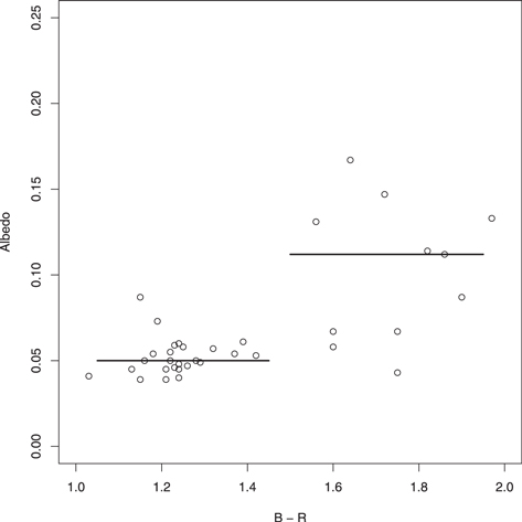
Figure 3. Albedos and optical B − R color of 31 Centaurs. The horizontal line segments mark the median albedos of the gray and red Centaur groups. This is an update of Figure 8 in Tegler et al. (2016). The Y axis range matches that of the range in that Figure 8. The Wilcoxon test shows a definite difference between the median albedos of the gray and red Centaurs (p = 8.5 × 10⁻⁵).
Download figure:
Standard image High-resolution imageHow do the albedos of Centaurs compare with the albedos of Trojans and Hildas? We must keep in mind that the Centaurs are considerably more distant than the Trojans and Hildas, so we are sampling a different size range of objects. The median size of the Centaur samples is 70 km (gray) and 58 km (red), while the median size of the Trojan samples is 16 km and of the Hildas, 8 km. Table 2 show that the red Centaurs are definitively more reflective at V wavelengths than any of the Trojan or Hilda samples. On the other hand, the gray Centaur sample albedo median is not statistically different from any of the Trojan samples. In particular, the median albedo of the gray Centaurs is almost the same as that of the L5 background. The median gray Centaur albedo is about 10% less than that of the L4 background, but the difference is not statistically significant with the current samples. Figure 4 shows the albedo distributions of gray and red Centaurs and L4 and L5 Trojans. The gray Centaur sample is ∼10% more reflective than the Hilda background and also the (153) Hilda family, but the significance is not particularly high (p-values around 0.01 to 0.05 depending on which sample is used). The gray and red Centaurs are statistically more reflective than the very dark (1911) Schubart family Hildas.

Figure 4. Albedos of (a) Trojan L5 background, (b) gray Centaurs, (c) Trojan L4 background and (d) red Centaurs. The medians are marked with vertical lines. For the Trojans, the albedos are from the mixed H samples. The gray Centaurs have a median albedo similar to the L5 background, but the median gray Centaur albedo does not differ in a statistically significant manner from either the L5 or the L4 backgrounds with the current sample. The red Centaurs have a significantly higher median albedo than the other three samples shown.
Download figure:
Standard image High-resolution image4.2. Jovian Trojans
Figure 5 shows a comparison of the Trojan L4 and L5 background samples. The L5 median albedo is ∼10% darker than the L4 median. Although this is perhaps a small and subtle distinction, the large number of objects make the difference highly significant (p = 4 × 10⁻⁸ for the mixed H samples and p = 3.6 × 10⁻⁷ for the smaller Pan-STARRS only sample). For the Wilcoxon test skeptic, we compared the distributions of the logarithms of the albedos of the L4 and L5 mixed H samples using the normality- assuming t test. This gave a p-value of 1 × 10⁻⁷, again indicating an extremely significant difference in median albedos. Of course, these small p-values found by both the Wilcoxon and t tests represent a true difference between the samples only if the instrumental calibrations of the infrared and optical are stable between observations of the L4 and L5 samples, which are separated on the sky by ∼120° on average as seen from the Sun, and a larger angle as observed from the dark side of the earth.

Figure 5. (a) Histogram of albedos of Trojan L5 background objects. The shaded portion of the histogram shows A values derived from HPS, while the open portion (stacked on top of shaded) shows albedos derived from transformed HHor values. The solid vertical line marks the median of the albedo values for the shaded area, and the dashed line the median value for the total (open plus shaded) mixed H sample. (b) The same for the L4 background. The Wilcoxon test shows that the medians of these two samples differ at a very high level of significance. However, as discussed in the text, the modes of the distributions are almost equal, and the difference in medians may be due to a more reflective component in the L4 background.
Download figure:
Standard image High-resolution imageVisual inspection of Figure 5 suggests that the distributions may not be simply slightly shifted distributions of the same shape. We estimate the mode of each distribution by fitting a parabola to the population versus bin central albedo for the five bins centered on the most populous bin. The mode of the L4 distribution (0.0470) is actually trivially smaller than that of the L5 distribution (0.0477), although the the median of the L4 distribution is 10% larger than that of L5. The L4 distribution may have an enhancement of objects with ∼0.06 < A < ∼0.12 as compared with the L5 distribution, which would not affect the mode of the L4 distribution but that would increase the L4 sample median. Perhaps there is an almost identical "true background" in both clouds, but the L4 cloud has an additional more reflective component not found in the L5 cloud.
Figure 6 shows comparison of the albedo histograms of the (3548) Eurybates family and the L4 background objects. The (3548) Eurybates objects have a median albedo significantly darker than the L4 background, with p-values of 4 × 10⁻⁶ for the mixed sample and 3 × 10⁻⁴ for the Pan-STARRS only sample. The (3548) Eurybates family objects are contained in the L4 cloud, and so would presumably have been observed close in time and sky position with the L4 background objects. It is interesting to note that the (3548) Eurybates median is closer to that of the L5 background than the L4 background. Table 2 p-values comparing L5 background and (3548) Eurybates albedos show the Eurybates median slightly darker, but the p-value for the Pan-STARRS only comparison is 0.07, which does not indicate a difference, while the mixed sample p-value is 0.005, which is significantly greater than the p-value for the L4 background—Eurybates comparison. If the L4 background sample contains an additional brighter component raising the median albedo of that sample, perhaps the (3548) Eurybates sample median albedo is close to that of the "true background" Trojan albedo and the disagreement with the L4 background median arises from the brighter component in L4.

Figure 6. (a) Histogram of albedos of (3548) Eurybates family objects in the L4 cloud. (b) Albedos of L4 Trojan background. Shading and vertical lines are same as in Figure 5. The Wilcoxon test shows that the medians of these two samples differ significantly. However, as discussed in the text, the median of the (3548) sample is closer to the L5 background median.
Download figure:
Standard image High-resolution imageThe (4709) Ennomos family median albedo does not differ in a significant way from that of the L5 background in which the family is found. However, the number of objects in the (4709) Ennomos is small.
4.3. Hildas; Hildas Versus Trojans
Figure 7 compares the Hilda (1911) Schubart family objects with the Hilda background. As noted in Grav et al. (2012), the Schubart objects are definitely darker than the Hilda background. We find a p-value for the comparison of albedos of the Hilda background and (1911) Schubart family samples that is "off the charts" (p < 2.2 × 10⁻¹⁶).

Figure 7. (a) Histogram of albedos of (1911) Schubart family objects. (b) Same for the Hilda background sample. Shading and vertical lines are same as in Figure 5. The Wilcoxon test shows that the medians of these two samples differ at an extremely high level of statistical significance (p < 2.2 × 10⁻¹⁶).
Download figure:
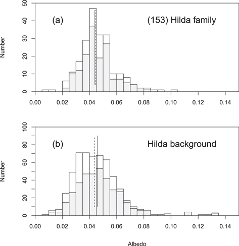
Standard image High-resolution imageFigure 8 compares the albedos of the objects in the (153) Hilda dynamical family with the albedos of the Hilda background. The p-values indicate that there is no statistically significant difference between the median albedo of the (153) Hilda family and the Hilda background for the samples studied here. This conclusion differs from Grav et al. (2012), who find that the (153) Hilda family has a higher albedo than the full Hilda population.
Figure 8. (a) Histogram of albedos of (153) Hilda dynamical family objects. (b) Same for the Hilda background sample. Shading and vertical lines are same as in Figure 5. The Wilcoxon test shows that the medians of these two samples do not differ in a statistically significant way.
Download figure:
Standard image High-resolution image
Table 2 p-values show that the Hilda background and (153) Hilda family are definitely darker than either the L4 or L5 Trojan background samples. Depending on which samples are used, the Hildas are 15%–25% less reflective than the Trojans. This is in broad agreement with the results of Grav et al. (2011) and Grav et al. (2012), who find an overall mean albedo of 0.07 for Trojans and 0.055 for Hildas, implying that the Hildas are 21% less reflective than the Trojans. The albedos given by Grav et al. (2011, 2012) are systematically higher than ours, due primarily, we believe, to their overestimate of optical brightness due to their use of Horizons H values, as discussed earlier. Correcting their mean albedos (0.07 and 0.055) for an optical overbrightness of 0.35 mag results in albedos of 0.05 for Trojans and 0.04 for Hildas, in fairly good agreement with the typical albedos presented in this paper.
5. Discussion
The combination of diameters from satellite thermal measurements and the rapidly increasing amount of accurate optical photometric data from surveys such as Pan-STARRS allows for unprecedented quantities of accurate albedo determinations for minor solar system bodies. In this paper we have presented a preliminary look at the data on a specific set of objects in the middle solar system: Centaurs, Hildas and Jovian Trojans. We find a number of potentially interesting phenomenological results. (1) We confirm and strengthen, using better HV values, our previous conclusion that red Centaurs (B − R > 1.45) have significantly higher albedos than gray Centaurs. The median albedo of the gray Centaur sample is about the same as that of the L5 Trojan background sample, but the present relatively small sample does not differ in a statistically significant manner from either the L5 or the L4 Trojan background samples. These results suggest the possibility of a common origin for the Trojans and the gray Centaurs. (2) The median L5 Trojan cloud albedo is about 10% darker than that of the L4 cloud at a very high level of statistical significance, but the modes of the two distributions are almost identical. We suggest that this may be due to the presence of an additional component with A ∼ 0.09 in the L4 cloud, which is not in the L5 cloud. (3) The (3548) Eurybates family is about 16% darker than the Trojan L4 cloud it resides in at a reasonably high significance level. The (3548) Eurybates median albedo is similar to that of the Trojan L5 cloud. The disagreement with the L4 cloud albedo may be due to the L4 cloud having a median albedo brighter than the true background, rather than the Eurybates family being darker than the Trojan background. (4) The (1911) Schubart dynamical family of Hildas is clearly darker than any other sample studied, and is about 30% darker than the Hilda background at an extremely high level of statistical significance. (5) The (153) Hilda dynamical family sample does not differ significantly in albedo from the Hilda background sample.
Any interpretation of these results obviously depends on the factors that determine the visual albedos of these types of bodies. Obviously surface chemical composition must play a major, if not dominant role. But other factors, such as surface physical properties (grain size, roughness) and surface impact and radiation exposure histories might also play important roles. We hope that studies such as ours, combined with detailed studies of individual bodies, both by remote sensing and eventual spacecraft visits, will help disentangle the factors that are important in determining the albedos of these objects.
We offer some speculation on the big picture of the albedos of gray Centaurs, Jovian Trojans, and Hildas. Perhaps these bodies all started out from the same source region, with similar compositions of ice and minerals. How might we explain the similar albedos of the gray Centaurs and Trojans and the significantly darker albedo of the bulk of the Hildas? The Hildas come closer to the Sun as compared to Trojans and Centaurs, resulting in higher solar radiation and, as argued below, significantly higher collisional flux. The typical Hilda has an orbit with a = 3.97 au and e = 0.2, while the typical Trojan has a = 5.2 au, e = 0.05. Using the equation relating time averaged solar flux and orbital parameters (Mendez & Rivera-Valentin 2017), these orbital parameters imply that the Hildas have a time averaged solar flux 1.75 times that of the Trojans. Due to the significant orbital eccentricity of the Hildas, the ratio of the peak (at perihelion) solar flux for a typical Hilda is 2.4 times that for a Trojan. The typical Hilda reaches a heliocentric distance of 3.18 au at perihelion. A plot of asteroid orbital element distributions9 shows a very significant asteroid population density in the main belt zone III region that extends to a ∼3.27 au. At perihelion, a Hilda with typical orbit will pass through this region with a velocity about 1.5 km s−1 relative to the circular velocity of objects at that radius. The resulting impacts of the Hildas and main belt asteroids and asteroid collisional debris, perhaps coupled with the increased solar flux near perihelion, could conceivably act to remove significant amounts of ice from the Hilda surface layers. This process is sometimes called gardening in the context of asteroid surface modification. Gardening plus solar radiation can darken icy surfaces (de Pater & Lissauer 2015). This might lower the average albedo of the Hildas as compared with initially very similar Trojans and gray Centaur objects. The gray Centaurs and Trojans would have much less gardening and solar radiation, so their albedos may be little changed over Gyr. The (3548) Eurybates and (153) Hilda dynamical families might be similar in origin and history to their background populations. In this general scenario, it is not obvious how the very dark (1911) Schubart family would fit in, but perhaps they are true interlopers.
We are grateful to the NASA Solar System Observations Program for support of the Centaur observations used in this paper.
Footnotes
- 4
- 5
- 6
- 7
- 8
- 9