

Abstract
Exact solutions are presented of the Klein–Gordon equation of a charged particle moving in a transverse monochromatic plasmon wave of arbitrary high amplitude, which propagates in an underdense plasma. These solutions are expressed in terms of Ince polynomials, forming a doubly infinite set, parametrized by discrete momentum components of the charged particle's de Broglie wave along the polarization vector and along the propagation direction of the plasmon radiation. The envelope of the exact wavefunctions describes a high-contrast periodic structure of the particle density on the plasma length scale, which may have relevance in novel particle acceleration mechanisms.
Export citation and abstract BibTeX RIS
1. Introduction
Analytic solutions of the wave equations of charged particles in the presence of strong radiation fields (such as those produced by high-intensity lasers) have played a crucial role in the description of multiphoton processes (Fedorov 1997). It is known that the Volkov states of an electron or other charged particle, being the exact solutions of the Dirac equation (Wolkow 1935), Klein–Gordon equation (Gordon 1927) or Schrödinger equation (Keldish 1964, Bunkin and Fedorov 1965), have long been an important theoretical tool in the study of these processes. Soon after the advent of the laser, these solutions were applied to describe various strong-field phenomena beyond the perturbative regime (see Brown and Kibble 1964, Eberly 1969, Neville and Rohrlich 1971, Gitman et al 1975, Ritus and Nikishov 1979 and Bergou and Varró 1980), and their study has nowadays received a renoved interest (see e.g. Panek et al 2002, Zakowicz 2005, Salamin et al 2006, Peatross et al 2007, Musakhayan 2008, Ehlotzky et al 2009, Boca 2011, and Harvey et al 2012). In the relativistic regime the closed analytic form of this set of states relies on the vacuum dispersion relation of the electromagnetic (EM) plane wave. If the EM field propagates in a medium (with a real index of refraction nm ≠ 1), or the strong laser field is modelled by a time-periodic electric field, then the relativistic wave equations can be reduced to Mathieu or Hill equations (see Nikishov and Ritus 1967, Nikishov 1970, Narozhny and Nikishov 1974, Becker 1977, and Cronström and Noga 1977). This problem, in the context of pair creation processes in strong fields, has again received a considerable theoretical interest recently (see e.g. Narozhny et al 2004, Popov 2004, Dunne 2004, 2009, and Müller and Müller 2012). Except for some special cases, the solutions cannot be expressed in a closed finite form; they are related to higher transcendental functions. In this context it is interesting to note that if one describes a Schrödinger particle, interacting with an EM plane wave in vacuum, beyond the dipole approximation (by taking exactly into account the spatial variation of the field), then one also encounters Mathieu or Hill equations, with their associated stability charts and band structures (Bergou and Varró 1981). However, the occurrence of such band structures for the momenta has been shown to be a result of the inconsistent use of the nonrelativistic description for high-intensity fields, as has been pointed out by Drühl and McIver (1983).
In the present letter we show that there are exact closed form solutions of the Klein–Gordon equation of a charged particle moving in a monochromatic classical plane EM field in a medium of index of refraction nm < 1. Recently we have solved the analogous problem for a Dirac particle (Varró 2013), and encountered (by now unknown) finite complex Fourier sums. The solutions to be derived in the forthcoming section are expressed in terms of known trigonometric polynomials; the Ince polynomials. Their arguments are integer or half-integer multiples of the EM wave's phase, and they form a doubly infinite discrete set of solutions labelled by two integer quantum numbers. This latter property is a completely new feature in comparison with both the Gordon–Volkov states (in vacuum) parametrized by continuous four momenta, and the Mathieu-type solutions characterized by a band structure of the allowed regions of the disposable parameters. We note that in mathematical physics Ince polynomials also appear in the description of various other systems. For instance, if one separates the two-dimensional harmonic oscillator wavefunction by using elliptic coordinates (Boyer et al 1975) then the eigenfunctions are products of Ince polynomials.
In section 2, during the course of the derivation of Ince's equation from the Klein–Gordon equation, we also make a brief comparison with the method leading to the usual Volkov states or to the Mathieu-type wavefunctions. Section 3 is devoted to the determination of the real polynomial solutions, which are associated with the eigenvalue problem of special finite tri-diagonal matrices. The solutions coincide with the Ince polynomials, labelled by two integer quantum numbers, which represent a quantized spectrum of the electron's momentum components along the (linear) polarization direction and along the propagation direction of the laser field. In section 4 we shall summarize the main mathematical properties of the solutions obtained, and few physical implications associated with them will be mentioned. In general, more emphasis shall be placed on the existence and analytic form of these solutions than on physical and numerical results. However, in section 4 some numerical examples will also be presented, just for illustration purposes. In section 5 a brief summary with conclusions closes our letter.
2. On the Volkov-type solutions and on the Mathieu-type solutions of the Klein–Gordon equation
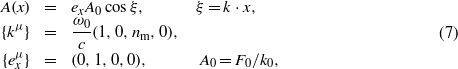
In an external electromagnetic field characterized by the four-vector potential A(x), the Klein–Gordon equation of a particle of charge e and of mass m has the form1

where c is the velocity of light in vacuum, and ħ is Planck's constant divided by 2π. In a medium of index of refraction nm, a general transverse electromagnetic plane wave of wavevector k can be represented by a vector potential
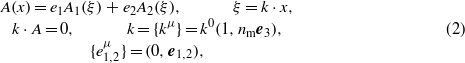
where {e1,e2,e3} form a right system of mutually orthogonal unit vectors. In principle, the scalar functions A1,2(ξ) in (2) may have arbitrary form (satisfying, of course, certain regularity conditions). For a purely monochromatic field A1,2(ξ) are simple sine and cosine functions and k0 = ω0/c, where ω0 = 2πν0 is the circular frequency. In the case of a general plane EM field, the solutions can be expressed in a simple closed form Gordon (1927). By taking a modified de Broglie plane wave, associated with a four-momentum parameter pμ, we have
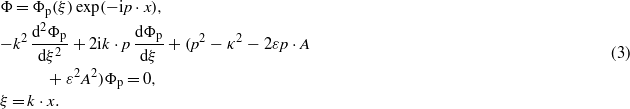
In vacuum (nm = 1, k = k0(1,e3), k2 = 0) the factor of the second derivative in (3) is zero, and the remaining first-order equation can be directly integrated, yielding the Gordon–Volkov states,
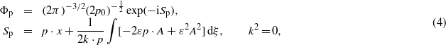
where Sp is the classical action divided by ħ. Equation (4) displays the generic structure of the Gordon–Volkov type states, the exact solutions of the Klein–Gordon equation of a charged particle interacting with a plane electromagnetic wave in vacuum. Concerning the basic mathematical properties of these solutions, see the early papers by Brown and Kibble (1964), Eberly (1969), Bergou and Varró (1980), and the recent work by Boca (2011).
The analysis becomes more complicated if one considers the interaction with a plane wave propagating in a medium of index of refraction nm ≠ 1. This is due to the presence of the non-vanishing second derivative in (3), since now  . In this case we can avoid the appearance of the first derivative in (3), by using the following Ansatz,
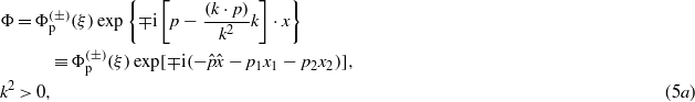
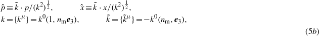
where the ambient sign ∓ refers to the 'positive and negative energy solutions'. The plane wave factor in the first equation in (5a) has also been written as ![$\exp [\mp \mathrm{i}(-\hat {p}\hat {x}-{p}_{1}{x}_{1}-{p}_{2}{x}_{2})]$](https://content.cld.iop.org/journals/1612-202X/11/1/016001/revision1/lpl488446ieqn103.gif) , where p1 = e1⋅p and p2 = e2⋅p are the transverse momentum components. We have introduced the 'complementary wavevector'
, where p1 = e1⋅p and p2 = e2⋅p are the transverse momentum components. We have introduced the 'complementary wavevector'  (
( and
and  ), with the help of which one can derive
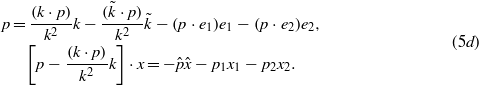
If  , then
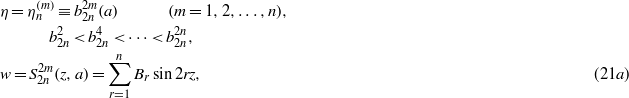
  is space-like, and
  plays the role of a momentum component conjugated to the 'position variable'
  (see e.g. Becker 1977). Thus, the Ansatz in (5a) means a separation of variables, where
  , p1 and p2 are 'three-momentum type parameters', and pξ = (k⋅p) may be said to be an 'energy-type parameter'. This latter parameter pξ does not explicitly show up in the solution, because (pξ/k2)kμ is subtracted from pμ (see (5d)).
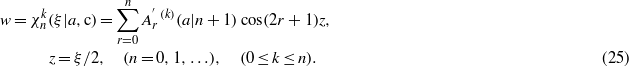
In the case of a right-circularly polarized monochromatic plane EM wave, for instance, one has Acir(x) = A0(excosξ + ezsinξ),  constant, and one immediately obtains a Mathieu equation for the modulation function
  , which we write in the standard form (Meixner and Schäfke 1954)
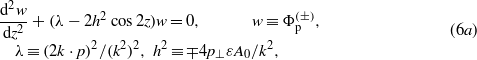

(See e.g. Becker 1977, and Cronström and Noga 1977.) We note that the two terms κ2 and  in the mass–shell relation are usually combined to
 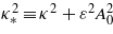 , which is the intensity-dependent mass shift
 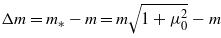 , where μ0 = eF0/mcω0 is the well-known dimensionless intensity parameter (see e.g. Brown and Kibble 1964, and the recent works by Harvey et al 2012, and Müller and Müller 2012).
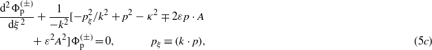
Henceforth, in equation (1) and in (5c) we specialize A = A(ξ) to represent a monochromatic linearly polarized plane wave,
where ω0 = 2πν0 is the circular frequency and F0 denotes the amplitude of the electric field strength. This is an x-polarized wave which propagates in the positive y-direction in the medium, i.e. the explicit form of the argument of the cosine is ξ = k⋅x = ω0(t − nmy/c). The differential equation (5c) for the modulation function  can be brought to the form,

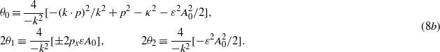
In (8a) we have defined the independent variable z = ξ/2 (as is usual in the theory of differential equations with periodic coefficients), and followed the standard notations for the parameters θ0,1,2. According to (8a), in the case of a linearly polarized monochromatic wave (7), the modulation function  satisfies the so-called Whittaker–Hill equation (or Hill's three-term equation), because now
  constant. If one attempts to solve this equation in terms of a trigonometric series, that procedure leads to five-term recurrence relations between the coefficients, in contrast to the three-term expressions encountered with the Mathieu equation. Thus, the standard procedure (the technique of continued fractions) cannot be taken over from the theory of Mathieu equations. In looking for finite-term solutions, we overcome this difficulty by using the transformation, originally due to Ince (see Arscott 1964, and references therein). This is the basic new element in our present approach. In the spirit of this method, in order to solve (8a), we proceed by introducing the following Ansatz for
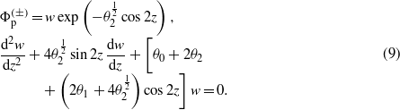
By using a more condensed notation, from (9) we receive the standard form of Ince's equation,


The second equation of (10c) from the first one has been derived by using the relations
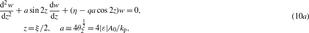
which is valid for an arbitrary four vector pμ, where  and pξ have been defined in (5b) and (5c), respectively. In obtaining (10a)–(10c) from (8a) and (8b) we have taken a negative test charge (electron; ε < 0), and considered 'positive solutions'. Note that equation (10a) is unchanged under the simultaneous substitutions z → z + π/2 and a → −a, thus we need not consider the case ε > 0 and ε < 0 separately. In (10b) we have introduced the new parameters q = (2px/kp) − 1 and
 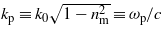 , where the subscript 'p' in the latter symbol refers to the word 'plasma', though at the present stage we do not need to specify the nature of the medium (in section 4 we shall deal with this interpretation).
In the rest of the present letter we shall study the general equation (10a); however, we shall not carry out a complete analysis of this equation, which has a quite unexplored infinite set of transcendental solutions. Our analysis is restricted to the special class of solutions, the (finite) Ince polynomials, which form a subset of all solutions. The exceptional feature of these solutions is that they form a doubly infinite countable set, corresponding to discrete values of the transverse and longitudinal momentum parameters.
3. Basically periodic, finite solutions of the Klein–Gordon equation
In section 2 we have derived Ince's equation (10a) for the modulation function of a de Broglie plane wave solution of the original Klein–Gordon equation (1). In order to obtain periodic finite solutions we follow the procedure explained in chapter 7 of Arscott (1964). At this point we would like to note that we have already used an analogous method for obtaining a new class of exact solutions of the corresponding Dirac equation, where, in contrast to (10a), we have encountered a complex equation, whose solutions turned out to be finite complex Fourier sums (Varró 2013). Though the method itself used there is analogous to that we are now using, the complex wavefunctions obtained have quite different properties from those of the real Ince polynomials, which we are deriving in the present section.
Let us first expand the solution of Ince's equation (10a) as a cosine series,
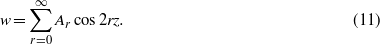
After substitution (10a), we have the recurrence relations for the unknown coefficients,


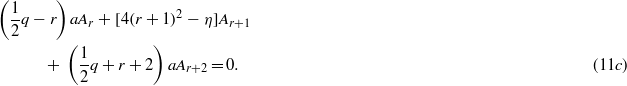
The parameter q has been defined in (10b), according to which q = (2px/kp) − 1. If q is a positive even integer, q = 2n, and if moreover η is chosen so that An+1 = 0, then, according to (11c) with r = n we have An+2 = 0 also, thus, successively An+3 = An+4 = ⋯ = 0. This means that the series terminates with the term Ancos2nz, and (11a)–(11c) becomes


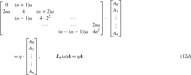
The solution of this system corresponds to a standard algebraic eigenvalue problem of the following tri-diagonal (n + 1) × (n + 1) matrix.
Following Arscott's notation, we use the symbol for the tri-diagonal matrix,
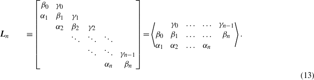
With this notation the tri-diagonal matrix, Ln(a) in (12d) is represented by the following symbol
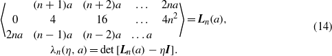
In (14) we have also introduced the characteristic polynomial λn(η,a) associated with the eigenvalue problem, where I is the (n + 1) × (n + 1) unit matrix. The eigenvalues are given by the zeros of the characteristic polynomial 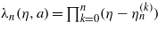 , in our case they are all real, and they are all simple roots of the equation λn(η,a) = 0. This is a consequence of the following lemma quoted on page 21 by Arscott (1964).
Lemma 1 (a) Let the numbers αi,βi,γi be all real, each product αi+1γi positive, and let Ln denote the tri-diagonal matrix above (13), all other elements being zero. Then the latent roots of Ln are all real and different.
(We have inserted '(13)' into the quotation, in order to refer our equation (13) above.) There are (n + 1) real linearly independent eigenvectors  , associated with the eigenvalues
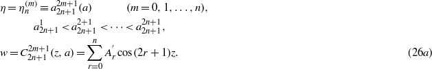
 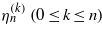 . According to the above considerations, if q = 2n, i.e. if
 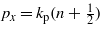 , then the potentially infinite cosine series in (11) reduces to the Ince polynomial
These solutions may be called 'even solutions' of (10a). In the notation  the letter 'c' refers to the word 'cosine', and in
  the second argument refers to there being n + 1 sets of the coefficients (eigenvectors), and the superscript labels the kth such set.
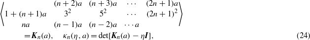
We note that Ince introduced the following notations for the ordered roots of λn(η,a) = 0 and for the associated polynomials (Arscott 1964)
These functions are normalized and they are orthogonal to each other,


The latter orthogonality relation can be derived in the usual way, by using (8a), (9) and (10a). The wavefunction in equation (15) is the Ince polynomial  displayed in (16a),
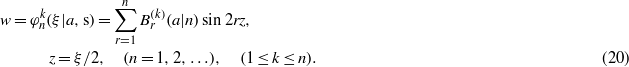
Still for q an even positive number, q = 2n, there are also odd solutions of Ince's equation (10a). Let us now expand the wavefunction as a series of sines,
The recurrence relations for the unknowns have the same structure as equations (12a)–(12c), except that the first is omitted, and we take B0 = 0,

If q is a positive even integer, q = 2n, and if moreover η is chosen such that Bn+1 = 0, then, according to equation (17b), with r = n we have Bn+2 = 0 also, thus, successively Bn+3 = Bn+4 = ⋯ = 0, which means that the series terminates with the term Bnsin2nz,


The solutions of this system are determined by solving the eigenvalue problem of the n × n tri-diagonal matrix
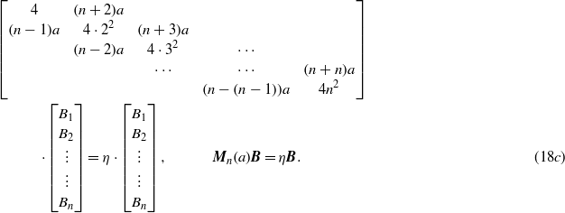
By using the condensed notation, as in (14), we write
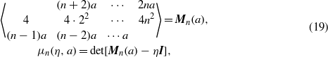
where I means here the n × n unit matrix. The eigenvalues are the roots of the characteristic polynomial, i.e. 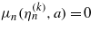 . The matrix Mn(a) in (19) also satisfies the conditions of the above lemma, thus the eigenvalues are all real and simple. In this way, we have found that, if q = 2n, i.e. if
  , then the potentially infinite sine series in (17) reduces to the following Ince polynomial
These solutions may be called 'odd solutions' of (10a). In the notation  the letter 's' refers to the word 'sine', and in the coefficients
  the second argument shows that there are n sets of the coefficients (eigenvectors), where the superscript labels the kth such set. The properties of the 'even sine-type solutions' discovered have been summarized by Arscott (1964) in complete analogy with (16a)–(16c),


The 'even sine-type solutions' in (20) thus coincide with the corresponding Ince polynomials in (21a),

There are finite solutions with q being an odd number. Let us try to find these in the form
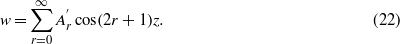
The coefficients satisfy the recurrence relations

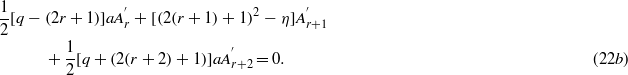
Let us assume that q is a positive odd integer, q = 2n + 1, and require that η is such that at r = n + 1 the coefficient  vanishes. Then, by putting r = n in (22b) we see that the first two terms on the left-hand side are zero, consequently
  vanishes, too, and all the higher index coefficient vanish—thus we have again a finite-term expression for the wavefunction. Accordingly, (22a) and (22b) are rewritten as


The characteristic numbers are solutions of the eigenvalue problem of the (n + 1) × (n + 1) tri-diagonal matrix
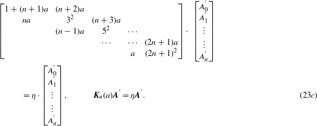
By using the condensed notation introduced in (13), we have
where I means the (n + 1) × (n + 1) unit matrix. According to the above lemma, the eigenvalues (the roots of the characteristic equation κn(η,a) = 0) are all real and different. We have shown that if q = 2n + 1, i.e. if px = kp(n + 1), then the potentially infinite cosine series in (22) reduces to the Ince polynomial
By using Ince's notation, the ordered roots of κn(η,a) = 0 and the associated polynomials are
The normalization condition and the orthogonality relation of  are the same as in (16b) and (16c),


The wavefunction in equation (25) can be expressed with the Ince polynomial  in (26a),
Finally, we study the 'odd sine-type solutions'
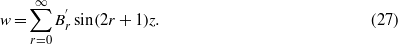

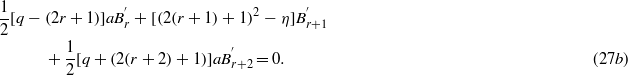
By using the same reasoning as above for an odd q = 2n + 1, from (27a) and (27b) we have


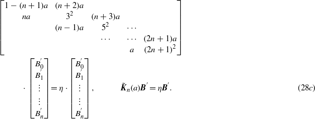
With the condensed notation introduced in (13), we have
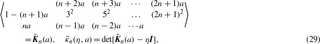
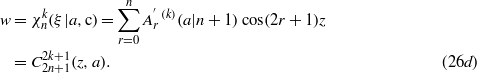
where I is the (n + 1) × (n + 1) unit matrix. As has been pointed out by Arscott (1964), the characteristic equation  is equivalent to κn(η, − a) = 0, where κn(η,a) has been defined in (24). To summarize this part of the section, we have found that if q = 2n + 1, i.e. if px = kp(n + 1), then the cosine series in (22) reduces to the Ince polynomial
By using Ince's notation, the ordered roots of  and the associated polynomials are
The normalization condition and the orthogonality relation of  are the same as in (26b) and (26c),


The wavefunction in equation (30) can be expressed with the Ince polynomial  in (31a),
According to (5a), (9), (10a), (15), (20), (25) and (30) the exact polynomial solutions of the Klein–Gordon equation (1) can be written as

For short, we have denoted the (Ince) polynomials (15), (20), (25) and (30), by the general symbol  . For each n-values (corresponding to a discrete set of transverse momenta 2px = (q + 1)kp), the coefficients of the polynomials given by (15), (20), (25) and (30), satisfy the inhomogeneous equations (12d), (18c), (23c) and (28c), respectively. There are n (or n + 1) real, linearly independent eigenvectors A(k), B(k), A'(k) and B'(k). The eigenfunctions associated with the eigenvalues
  form a doubly infinite set labelled by the integer numbers n and k. The eigenvalues are all real, and the eigenfunctions are real trigonometric polynomials, which coincide with the Ince polynomials, as has been explicitly displayed by (16d), (21d), (26d) and (31d). The possible values of the momentum parameter of the solutions are connected to eigenvalues
  by (10c). Since px is given (it is either
  or px = (n' + 1)kp, where n = 1,2,... and n' = 0,1,...), the relation (10c) determines n (or n') possible values for
  , which may be labelled as
  , where 0,1 ≤ k ≤ n. We note that for any value of the transverse momentum px = (q + 1)kp/2 (regardless of q is an integer or not) it is always possible to find a denumerably infinite set of basically periodic even solutions
  and odd solutions
  , associated with the eigenvalues
  and
and  , respectively (Arscott 1964). In the limit of small intensities (a → 0) these transcendental Ince functions go over to cosmz and sinmz. Research on the asymptotic behaviour of the so-called instability zones of Whittaker–Hill type equations, such as (8a), has recently led to new significant results (Djakov and Mityagin 2007), which may have importance in applying our solutions; however, the discussion of these is beyond the scope of the present letter.
We also note that an analogous new set of exact solutions of the corresponding Dirac equation have been recently found by us (Varró 2013), which are also expressed by finite trigonometric polynomials. However, these new polynomials are complex Fourier sums, whose interrelation with the Ince polynomials (which have an already well-developed theory) has not been explored.
4. Numerical illustrations of some basic properties of the new exact solutions
The investigation of various possible physical applications of the exact solutions (32) is out of the scope of the present letter. The emphasis has been on proving the existence and on constructing the general polynomial solutions. In the present section we shall only briefly discuss a possible physical background of these solutions, and give a few numerical illustrations.
Each of the solutions (32) contains the exponential factor exp[ − (a/4)cosξ], which can be expanded into an infinite Fourier series (Gradshteyn and Ryzhik 1980 or Abramowitz and Stegun 1965),
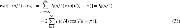
where Il(z) denotes the modified Bessel functions of first kind of order l. This means that, though the polynomials  are finite-term expressions, the complete wavefunction (32) contains all the higher harmonics of the fundamental frequency. If a is large, then this function is peaked at the points ξ = π − 2kπ (k being an arbitrary integer) with an exponentially large contrast, as is shown in figure 1.

Figure 1. Normalized square of the envelope function, exp[ − (a/2)cosξ], in the wavefunction (32) for two values of the fundamental parameter a = 4|ε|A0/kp. (a) a = 4, (b) a = 14. At the centre of the base interval −π ≤ ξ ≤+ π the 'probability density' is practically zero; this 'void region' represents a sort of 'bubble'.
Download figure:
Standard image High-resolution imageFigure 1 illustrates the simple fact that the exponential factor exp[ − (a/2)cosξ] behaves as an envelope on the base interval, rather than showing some structured modulations, which might be expected on the basis of its high harmonic content, according to (33). For large a, the spectrum, governed by the modified Bessel function of first kind, is practically independent of the index l, owing to the asymptotic behaviour ![${I}_{l}(z)=({\mathrm{e}}^{z}/\sqrt{\pi z})[1+\mathrm{O}(1/z)]$](https://content.cld.iop.org/journals/1612-202X/11/1/016001/revision1/lpl488446ieqn344.gif) (Abramowitz and Stegun 1965).
(Abramowitz and Stegun 1965).
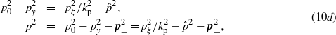
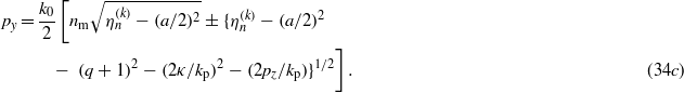
The differential equation (10a) has led to a two-parameter eigenvalue problem, where we have considered a = 4|ε|A0/kp as a 'fundamental parameter', and 2px = (q + 1)kp and η were 'disposable parameters'. We have seen that the condition q + 1 = 2n leads to even cosine-type and even sine-type solutions, and q + 1 = 2n + 1 to odd cosine-type and odd sine-type solutions. On the basis of the two equivalent forms of the eigenvalues η in (10c), the momentum parameters can be expressed as
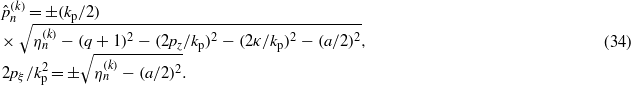
The second equation of a simpler form in (34) has been obtained by imposing (in addition) the free mass–shell condition (p2 = κ2) for the momentum parameter pμ, where the definition of pξ in (10c) has also been used. The eigenvalues  are the roots of the characteristic equations λn(η,a) = 0, μn(η,a) = 0, κn(η,a) = 0 and
  , where the characteristic polynomials have been defined in (14), (19), (24) and (29). In general, p0 and py can be expressed as
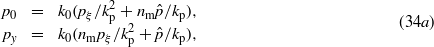
regardless of any constraints. If we impose the free mass–shell condition p2 = κ2, then, from (34), by choosing the positive sign in the second equation, we have
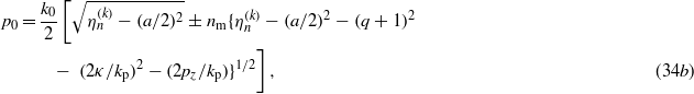
According to (34), the parameter pξ (which reduces to the energy pξ/k0 → p0 in the limit nm → 0 of the pure electric field case) can only be real if η ≥ a2/4. For these eigenvalues, 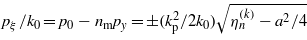 would correspond to a sort of 'gap state', because it can happen that −mc2 < ħcp0 <+ mc2 in the pure electric case. On the other hand, one has to keep in mind that, in general, the parameters p0 and py are not 'good quantum numbers' in the case of the interaction we are considering. Besides the transverse momenta px = kp(q + 1)/2 and pz, only the 'longitudinal combination'
 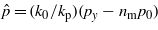 is a constant of motion, and p0 and py separately have no immediate physical meaning. Moreover, not all the eigenvalues give physically acceptable solutions of the Klein–Gordon equation. If
  becomes purely imaginary, then the wavefunctions necessarily contain the exponentially growing factor
 ![$\exp [\pm \vert \hat {p}\vert ({k}_{0}^{2}/{k}_{\mathrm{p}}^{2})(y-{n}_{\mathrm{m}}{x}_{0})]$](https://content.cld.iop.org/journals/1612-202X/11/1/016001/revision1/lpl488446ieqn382.gif) in the space-like direction
in the space-like direction  . This would not be an acceptable solution, except for the case when the interaction is limited in a finite space–time region. In the optical range (2κ/kp)2 is on the order of (106)2, thus η must be as large, in order to have a real square root and propagation constant in (34). We note that, alternatively, the laser-modified mass–shell relation
  may also be prescribed, where
 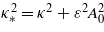 contains the intensity-dependent mass shift (see e.g. Harvey et al 2012 or Müller and Müller 2012). In this case the first equation of (34) remains the same (because it does not depend on any restriction for the momentum parameter). The right-hand side of the second equation of (34) becomes different, it is then
 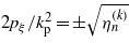 .
.
Concerning possible physical applications of the exact solutions embodied in (32), one has to keep in mind that, in general, the index of refraction depends on the frequencies of the spectral components of the radiation field, i.e. nm = nm(ω). The assumed dependence of the field amplitudes merely through the combination ξ = k⋅x = k0c(t − nme3 ⋅r/c) with some constant nm, is, of course, an idealization. The monochromatic field is usually meant to model a real quasi-monochromatic field having a very small spectral spread Δω ≪ ω0 around some central frequency ω0 = ck0, and in the present letter we assume that the associated variation of the index of refraction is negligible in this spectral range, i.e. Δnm ≪ nm. For example, our analysis may be relevant for the description of the interaction of a relativistic electron with a strong laser field propagating in an underdense plasma. In the case when the Drude free electron model applies, the index of refraction may well be approximated by the formula 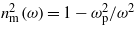 , with
 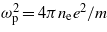 , where ωp is a real plasma frequency, where ne is the density of the plasma-electrons. If
  , then Δnm/nm < Δω/ω is satisfied for all such frequencies, thus in case of Δω/ω ≪ 1 the relative spectral variation of the index of refraction is also negligible, Δnm/nm ≪ 1. Under these conditions, the vector potential displayed in (2) can be a faithful representation of a quasi-monochromatic radiation field in a homogeneous plasma medium. The invariant square (effective mass of the EM field) of the propagation vector
 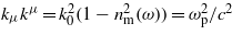 does not depend on the circular frequency ω of the laser field.
The fundamental parameter a can be expressed in terms of various combinations of parameters characterizing the applied monochromatic field and the medium. Taking the free electron model of a plasma medium, with a dielectric permittivity 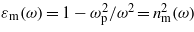 , the electromagnetic plane wave under discussion has the dispersion relation
 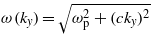 , with ky = nmω/c, corresponding to the phase ξ = ω(t − nmy/c) of the laser field. In this case the parameter a can be written as the work done by the electric force along the plasma wavelength divided by the photon energy. The ratio of the photon density and the electron density also naturally appears,
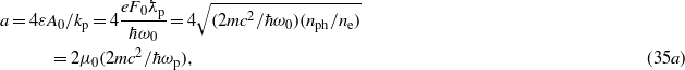
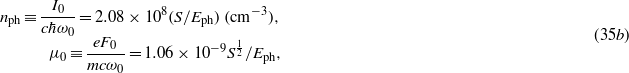

We have used the definition  of the 'plasma wavenumber' in (10b), and introduced the true plasma frequency ωp. For example, the electron density ne = 7.242 × 1020 cm−3 corresponds to the plasmon energy ħωp = 1 eV (in which case the plasma wavelength is λp = 1240 nm). In the numerical expressions of the photon number density nph and of the well-known 'dimensionless intensity parameter' μ0 (which nowadays is also called 'scaled vector potential'), the quantities S = I0 (W cm−2)−1 and Eph = ħω0 (eV)−1 measure the intensity in watts per square centimetre and the photon energy in electron volts, respectively. For a Ti:Sa laser with λ0 = 795 nm we have ħω0 = 1.563 eV > ħωp, which means that this radiation freely propagates in the underdense plasma, with the phase velocity c/nm and group velocity cnm. In this case a = 2 × 10⁶μ0 and μ0 = 6.782 × 10⁻¹⁰S1/2, showing that for optical frequencies the parameter a is by six orders of magnitude larger than the usual intensity parameter μ0.

Figure 2. Eigenvalues associated with the four types of solutions (32a), for a = 14 and n = 20. We have taken ħωp = 1 eV and n = 20, i.e. the transverse momentum of the electron (in original units) is px = 20ħkp, where kp = ωp/c. The interaction with a Ti:Sa laser field of photon energy ħω0 = 1.563 eV and peak intensity I0 = 100 MW cm−2 has been considered as an example. The eigenvalues in (a), (b), (c), (d) are the roots of the characteristic equations λn(η,a) = 0, μn(η,a) = 0, κn(η,a) = 0 and  , where the characteristic polynomials have been defined in (14), (19), (24) and (29), respectively. Notice that in (a) there are 20 eigenvalues, and in (b)–(d) there are 21. We have not used Ince's ordering of the eigenvalues displayed in (16a), (21a), (26a) and (31a). The difference and comparison of the two numberings are explained in more detail in (e) and (f). Illustration of the difference between the numbering of the eigenvalues used in the present letter and that used by Ince, displayed in (16a), (21a), (26a) and (31a). As an example we show that in (a) above the smallest (negative) eigenvalues in (e) we have the indices k = 11, 14, 16 and 18 in our figure. On the other hand, according to Ince's convention, they would have indices m = 0, 1, 3 and 4. The largest eigenvalue has index k = 0, which corresponds to the largest m = 20 in Ince's numbering. The arrows symbolize the increase of the integer index from 0 to 20. On the abscissa only the values of k = 0,1,...,20 are shown. We have followed the numbering of the eigenvalues as they are ordered by the program Wolfram Mathematica©8 (Copyright 1988–2010 Wolfram Research, Inc.). An additional reason for using this numbering is that we have observed that in the 'oscillatory part' of the spectrum (as is emphasized in (e) by the arrows), with negative values, the wavefunctions are qualitatively different from those belonging to the 'monotone part'. This is clearly illustrated in figures 5 and 6.
Download figure:
Standard image High-resolution imageEven for a relatively moderate intensity of 100 MW cm−2 (S = 108), the value of a = 13.56 ≫ 1 is already quite large. In figure 1 we present illustrations for the eigenvalue spectrum in the case of such a moderate intensity, for which we assumed a = 14, and have taken n = 20. In a recent experiment Kiefer et al (2013) have used a Ti:Sa laser of intensity I0 = 6 × 10²⁰ W cm−2, in which case μ0 = 16.61 is well beyond the relativistic limit (μ0 = 1), and consequently a = 3.32 × 10⁷ is very large. We note that in such extreme cases there exist approximate analytic formulae for both the eigenvalues and for the Ince polynomials; however, in the present letter we do not have space to enter into these details.
In figure 3 we show the distribution of the harmonic strengths (such as ![$[{A}_{r}^{(k)}(a\vert n+1)]^{2}$](https://content.cld.iop.org/journals/1612-202X/11/1/016001/revision1/lpl488446ieqn442.gif) from (15)) in the expansion of the polynomial factors, in the case of the interaction with a Ti:Sa laser field of photon energy ħω0 = 1.563 eV and peak intensity I0 = 100 MW cm−2 in a plasma medium of electron density ne = 7.242 × 1020 cm−3 (ħωp = 1 eV). Of course, the complete physical spectrum may in principle be influenced by the exponential prefactor leading to the modified Bessel function series in (33), but in the present letter we would like to put the emphasis on the properties of the less-known polynomial factors. According to figure 3, these spectra are in general qualitatively different from each other. As the index k of the eigenvalue increases, the single-peaked structure gradually shifts from the higher harmonics to the lower harmonics. When the first negative eigenvalue is reached, then the harmonic distribution becomes oscillatory, and beyond this border oscillations are also present in the solutions belonging to positive eigenvalues. In figure 4 we give an overview of the harmonic spectra in figure 3.
from (15)) in the expansion of the polynomial factors, in the case of the interaction with a Ti:Sa laser field of photon energy ħω0 = 1.563 eV and peak intensity I0 = 100 MW cm−2 in a plasma medium of electron density ne = 7.242 × 1020 cm−3 (ħωp = 1 eV). Of course, the complete physical spectrum may in principle be influenced by the exponential prefactor leading to the modified Bessel function series in (33), but in the present letter we would like to put the emphasis on the properties of the less-known polynomial factors. According to figure 3, these spectra are in general qualitatively different from each other. As the index k of the eigenvalue increases, the single-peaked structure gradually shifts from the higher harmonics to the lower harmonics. When the first negative eigenvalue is reached, then the harmonic distribution becomes oscillatory, and beyond this border oscillations are also present in the solutions belonging to positive eigenvalues. In figure 4 we give an overview of the harmonic spectra in figure 3.

Figure 3. Strength ![$[{A}_{r}^{(k)}(a\vert n+1)]^{2}$](https://content.cld.iop.org/journals/1612-202X/11/1/016001/revision1/lpl488446ieqn29.gif) of the harmonic coefficients of the polynomial
of the harmonic coefficients of the polynomial  for four eigenvalues labelled by the upper index k = 0,9,15,20. We are considering the case when a = 14 and n = 20, and the input parameters are the same as in figure 2.
Download figure:
Standard image High-resolution image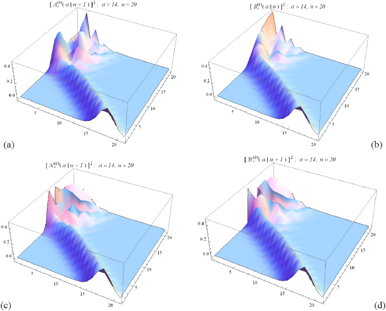
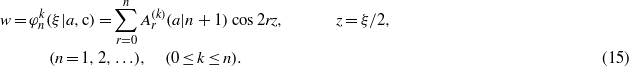
Figure 4. Overview of the strength of the harmonic coefficients on a three-dimensional list plot when a = 14 and n = 20. (a) ![$[{A}_{r}^{(k)}(a\vert n+1)]^{2}$](https://content.cld.iop.org/journals/1612-202X/11/1/016001/revision1/lpl488446ieqn36.gif) , (b)
, (b) ![$[{B}_{r}^{(k)}(a\vert n)]^{2}$](https://content.cld.iop.org/journals/1612-202X/11/1/016001/revision1/lpl488446ieqn37.gif) , (c)
, (c) ![$[{A}_{r}^{{^{\prime}}~(k)}(a\vert n+1)]^{2}$](https://content.cld.iop.org/journals/1612-202X/11/1/016001/revision1/lpl488446ieqn38.gif) and (d)
and (d) ![$[{B}_{r}^{{^{\prime}}~(k)}(a\vert n+1)]^{2}$](https://content.cld.iop.org/journals/1612-202X/11/1/016001/revision1/lpl488446ieqn39.gif) . The input parameters are the same as in figure 2. This figure summarizes the behaviour of these quantities as functions of the harmonic numbers (r = 0,1,2,...,20 on the left axis), for different eigenvalues (k = 0,1,2,...,20, which are drawn on the right axis). The discrete points are connected by a smoothened surface in order to guide the eye. For the lowest index k = 0 (or k = 1 in (b)) the distribution is concentrated to large r-values (left axis) in a single peak. For larger k-values the single-peak structure goes over to an oscillatory distribution.
. The input parameters are the same as in figure 2. This figure summarizes the behaviour of these quantities as functions of the harmonic numbers (r = 0,1,2,...,20 on the left axis), for different eigenvalues (k = 0,1,2,...,20, which are drawn on the right axis). The discrete points are connected by a smoothened surface in order to guide the eye. For the lowest index k = 0 (or k = 1 in (b)) the distribution is concentrated to large r-values (left axis) in a single peak. For larger k-values the single-peak structure goes over to an oscillatory distribution.
Download figure:
Standard image High-resolution imageIn figure 5 we illustrate the detailed temporal evolution of the even cosine-type wavefunctions, whose harmonic spectra have been shown in figure 3. Finally, figure 6 illustrates the temporal evolution of the even sine-type wavefunctions. The further numerical study of the exact solutions (32) is out of the scope of the present letter.

Figure 5. Shape of the even cosine-type polynomial solutions  for four eigenvalues labelled by the upper index k = 0,9,15,20. a = 14 and n = 20, where the input parameters are the same as in figure 2. These functions are finite sums of the cosine function cos2rz = cosrξ, and the harmonic spectra of these functions have been shown in figure 3.
Download figure:
Standard image High-resolution image
Figure 6. Shape of the even sine-type polynomial solutions  for four eigenvalues labelled by the upper index k = 1,9,15,20. a = 14 and n = 20, where the input parameters are the same as in figure 2. These functions are finite sums of the sine function sin2rz = sinrξ, as shown in (20), (21d) and in the summarizing equations (32), (32a).
Download figure:
Standard image High-resolution image
5. Summary
We have presented exact closed form solutions of the Klein–Gordon equation of a charged particle (electron or proton) moving in a monochromatic classical plane electromagnetic field in a medium of index of refraction nm < 1. These solutions have been expressed in terms of Ince polynomials, which form a doubly infinite set, belonging to discrete momentum components of the particle's de Broglie wave along the polarization vector and along the propagation direction of the EM field. The odd Ince polynomials are finite sums of cosines or sines of the half-integer multiples of the phase of the incoming field, thus they describe half-integer order higher harmonics.
We have considered the medium as an underdense plasma, in which case the transverse momentum of the test charge is an integer or half-integer of the plasma momentum kp = ωp/c, i.e. px = nkp or  , where ωp is the plasma frequency. The other quantum number determines the possible eigenvalues of the longitudinal energy–momentum parameter. The fundamental (input) parameter a (see (35a)), characterizing the strength of the interaction, is the work done on the charge by the electric force of the EM field along a plasma wavelength divided by the photon energy. In contrast to the well-known intensity parameter μ0 (see (35b)), which often appears in the theory of strong laser field matter interactions, this a is a quantum parameter, and it is typically by many orders of magnitudes larger than the former one. We have found 'void regions' (or 'bubbles') in the particle density, centred in the middle of the plasma wave cycle with an exponentially large contrast (ea/2). This behaviour of the density corresponds to the formation of a regular and periodic structure on the plasma length scale, and it may have relevance in the study of novel acceleration mechanisms (see e.g. Xia et al 2012, Mourou et al 2013, Pukhov et al 2012).
In section 2 we have derived the relevant Ince equation from the original Klein–Gordon equation, and made a brief comparison with the derivation of the usual Volkov states, and of the Mathieu-type wavefunctions in a medium. In section 3 we have derived the two even and two odd periodic, finite solutions, which coincide with the corresponding Ince polynomials. These solutions are associated with the eigenvalue problem of finite special tri-diagonal matrices equation (13) and (16a) and (16b). We have restricted our analysis only to these special class of solutions, proportional with polynomial expressions. They form a subset of all solutions of the Ince equation, including the transcendental Ince functions. In section 4 we have given some numerical examples for the relevant parameters appearing in the analysis, and presented numerical illustrations for the discrete eigenvalues, the temporal shape of the wavefunctions, and for the harmonic spectra which are associated with them.
Acknowledgments
This work has been supported by the Hungarian Scientific Research Foundation OTKA, Grant No. K 104260. The author thanks the referees for many valuable questions, comments and criticism, which have been answered, and taken into account in compiling the final version of the present letter.
Footnotes
- 1
The Minkowski metric tensor gμν = gμν has the components g00 =− gii = 1 (i = 1,2,3) and gμν = 0 if μ ≠ ν (μ,ν = 0,1,2,3). The scalar product of two four-vectors a and b is a⋅b = gμνaμbν, i.e. a⋅b = aνbν = a0b0 − a ⋅b, where a ⋅b is the usual scalar product of three-vectors a and b, and a2 ≡ aμaμ. Space–time coordinates are denoted by xμ, where x = {xμ} = (ct,r). The four-gradient is ∂ = {∂μ} = (∂/∂ct, − ∂/∂r), and its covariant components are ∂μ = ∂/∂xμ.