Abstract
Antarctic Survey Telescopes (AST3) are designed to be fully robotic telescopes at Dome A, Antarctica, which aim for highly efficient time-domain sky surveys as well as rapid response to special transient events (e.g., gamma-ray bursts, near-Earth asteroids, supernovae, etc.). Unlike traditional observations, a well-designed real-time survey scheduler is needed in order to implement an automatic survey in a very efficient, reliable and flexible way for the unattended telescopes. We present a study of the survey strategy for AST3 and implementation of its survey scheduler, which is also useful for other survey projects.
Export citation and abstract BibTeX RIS
1. Introduction
Intelligent robotic observations and massive synoptic sky surveys are advancing research in astronomy. In this new exciting era, we face both opportunities and challenges, one of which is to develop a comprehensive observing scheduler for large automatic sky surveys. A survey scheduler generates a complicated plan on how to conduct a survey, or specifically, which fields to observe and at what times.
Observing efficiency has increased greatly for modern telescopes with some robotic features, which are streamlining the traditional operations to minimize overhead during night observations. A number of successful systematic large-area sky surveys have been carried out, such as the Sloan Digital Sky Survey (SDSS, York et al. 2000) and the Two Micron All Sky Survey (2MASS, Skrutskie et al. 2006). Large data sets from these efforts have been shared with the entire astronomical community to answer fundamental astrophysical questions. In general, a telescope scheduling system for this kind of survey should only focus on optimizing the use of nighttime, minimizing overhead and maximizing effective exposure time.
High observing efficiency is especially required for time-domain sky surveys monitoring the time-variable sky over a large sky area and detecting rare transient objects in real-time. Surveys such as the SDSS Stripe 82 Supernova Survey (Frieman et al. 2008), the Subaru/XMM-Newton Deep Survey (Morokuma et al. 2008), the Deep Lensing Survey (Becker et al. 2004) and the Faint Sky Variability Survey (Huber et al. 2006) have mainly concentrated on selected areas of tens to hundreds of square degrees and have typically searched for specific types of transients, so those surveys are easy to schedule. However, other large-scale time-domain surveys, such as the Palomar Transient Factory (PTF, Law et al. 2009), the Catalina Real-Time Transient Survey (CRTS, Drake et al. 2009), the Panoramic Survey Telescope and Rapid Response System (Pan-STARRS, Hodapp et al. 2004), as well as the future Large Synoptic Survey Telescope (LSST, Ivezic et al. 2008), are monitoring thousands of square degrees of the time-variable sky with targets ranging from distant supernovae (SNe) to near-Earth asteroids. Since different types of transients occur on different time scales as well as at different sky locations, the scheduler for such a time-domain survey could be complicated. Besides the general issues related to telescope scheduling, it is also required to balance the survey areas and the survey cadences that have different time scales which could range from seconds to years for different types of transients.
Rapid response to follow-up observations has also been a key issue in time-domain astronomy. Large sky surveys can build large statistical samples of objects and identify variable objects or transients that need detailed follow-up studies. Multi-wavelength space missions can also identify transient targets, such as gamma-ray bursts (GRBs). These often require rapid optical follow-up, mostly from the ground.Modern telescopes with robotic features are particularly well suited for ambitious programs requiring prompt response to unpredictable or rare events. The follow-up can also be coordinated simultaneously with more telescopes on the ground and other facilities in space.
Moreover, in order to achieve continuous observations, some global networks have been built with small telescopes to cover different time zones, such as ROTSEIII (Akerlof et al. 2003), RAPTOR/Thinking Telescopes (Wren et al. 2002) and HATNet (Bakos 2012). Larger telescopes have also been robotized for rapid response to rare, fainter transient targets, such as the Liverpool Telescope (Steele et al. 2004) which is a 2.0m fully robotic telescope. Currently, the largest global network would be the Las Cumbres Observatory (LCO, Brown et al. 2013) which is operating eighteen telescopes, including 0.4m, 1m and 2m ones, around the world. It is able to track a target continuously without a gap in time, if weather permits. LCO has developed a very complicated scheduler to coordinate and optimize use of the telescopes across the network.
In the case of the Antarctic Survey Telescopes (AST3) running at Dome A, Antarctica, robotization of the telescope operation is not just an optimization, but a requirement. Dome A is the highest part of the Antarctic plateau, located at 77.56° E, 80.367° S. Because of its unique geographic and atmospheric conditions, Dome A is thought to be the best site for ground-based astronomy. Recent studies have demonstrated that Dome A is a good astronomical site in both optical and terahertz (e.g., Zou et al. 2010, Zhou et al. 2010, Hu et al. 2014, Shi et al. 2016).However, due to its remoteness, Dome A can only be reached once a year during the austral summer by the Chinese Antarctic Research Expedition (CHINARE) team. Unlike other robotic telescopes which can bemaintained during the day time, all instruments at Dome A are unattended for an entire year and must be run automatically with only limited communication bandwidth via Iridium satellites (Yang et al. 2009, Bonner et al. 2010). Therefore, besides challenges related to the hardware, a robust, well designed observing scheduler is also required for AST3, taking into account not only general issues related to a general robotic telescope, but also the special conditions at Dome A.
2. The AST3 System
AST3 consists of three 50 cm telescopes that utilize a modified Schmidt design (Cui et al. 2008, Yuan et al. 2010, Yuan & Su 2012). The mirror support structure is made of INVAR steel which has a low thermal expansion coefficient. When the temperature changes too much at Dome A, there is an active focusing mechanism to keep the image sharp. Two filters can be used for each telescope and they can be changed on-site during servicing. The telescope can move relatively fast with a speed range of 5'' ∼ 1° s−1 in both Right Ascension (RA) and Declination (Dec) directions. The pointing accuracy is < 30'' RMS and the tracking accuracy is < 0.5'' RMS within 2 minutes with no guiding (Yuan et al. 2016).
Each telescope is equipped with a single-chip large-format 10 k×10 k CCD camera with pixel size of 9 μm which results in a plate scale of 1'' pixel−1 for AST3. The camera has been designed to have no mechanical shutter to avoid possible mechanical problems at extremely low temperatures, therefore the CCD is operated in frametransfer mode in which only the central 5 k×10 k area is used for exposure, corresponding to a field-of-viewof 4.3 square degrees (1.466°×2.933°).
Table 1 lists some of the key parameters of AST3. The first and second AST3 telescopes were installed at Dome A in 2012 and 2015, respectively, and the third one is under construction. We have developed a specific observing scheduler for AST3 and it has been re-designed and optimized for the second telescope as part of the Operation, Control and Data System of AST3 (Shang et al. 2012).
Table 1. Main Technical Characteristics of AST3
| Aperture | 50 cm |
| Mount type | Equatorial |
| Slew speed (Max) | 1° s−1 |
| CCD type | Frame transfer |
| CCD size | 5 k × 10 k pixels (exposed area) |
| Field of view | 4.3 square degrees (1.466° ×2.933°) |
The survey of AST3 is carried out by a complicated software system ast3suite (Hu et al. 2016), which automatically takes care of everything that is part of the survey, including telescope pointing, CCD camera exposure, data archiving, data reduction, various logging, alerts, etc. For each telescope pointing, ast3suite asks the scheduler for the next field, and the scheduler is responsible for providing the best available field according to pre-defined rules of the survey.
3. Pre-defined Observing Modes
Although the aperture of AST3 is not large, its unique location at Dome A makes it especially powerful for timedomain astronomy.During polar nights, there can be continuous observations spanning 3–4 months with cadence ranging from seconds to months. This has never been attempted anywhere else on the ground.
The primary science drivers of AST3 are
- (1)Very early discovery of SNe and photometric follow-up of SNe in multi-colors;
- (2)Exoplanet search, especially very short-period ones, and light curves with time resolution of minutes to days;
- (3)Rapid follow-up of transients detected by other ground-based telescopes or space missions, such as GRBs.
Since from both SN survey and exoplanet search, AST3 is able to provide light curves at a time resolution of minutes to days, and possibly cover a period around 4 months at most, these data can also be used for general time-domain research.
Observing time is always precious, and a good scheduler can significantly increase the observing efficiency. There are several general factors we need to consider when designing the scheduler, including the survey area, observing cadence, slew speed/frequency of the telescope, airmass, sky background, etc. The scheduler needs to balance the importance of factors for different observing requirements and make decisions. In most cases, it is not clear that there would be quantitative weights for the above factors. In addition, a general scheduler may not be suitable for all cases. Therefore, considering the observing requirements, we have defined three observing modes based on their scientific requirements.
3.1. Supernova Survey Mode
The SN survey endeavors to monitor as many galaxies as possible with a preferred cadence of days depending on the capability of the telescope. Therefore, it needs to survey an area as large as possible. The survey area or fields of pointing are provided by the scientific group. The scheduler reads and updates a text file containing all the survey fields, one per line, with its ID, RA, Dec, priority, exposure information, etc.
For each pointing, AST3 takes three images with exposure time of 30–40 s each to remove cosmic rays in coadding as part of the real-time pipeline (Ma et al. 2017, in preparation). While the images are processed by the pipeline, the telescope can move and point to another field, therefore, each field takes about 2 minutes. Given the AST3's field-of-view, it can cover about 100 square degrees of the sky per hour. During the polar nights, we can easily survey 2000 square degrees repeatedly every day. To avoid contamination by the Milky Way, an obvious choice for the SN survey area would be in the high Galactic latitude region, so we can set a lower limit on the Galactic latitude. This can be done when defining the SN survey pointing fields, but we can also set this limit as a parameter in the configuration file of the scheduler.
There are several limits on the observed fields, including the limit on Galactic latitude, the limit on telescope pointing, and the limit on airmass or sky background, etc., as defined in Section 4.1. In order to minimize the telescope slew time, we certainly prefer to observe one field after another in a spatial sequence, and it is better to move the telescope in the RA direction first and reverse the direction after changing to the next closest Dec when one of the limits is reached.
For follow-up observations with AST3 itself, certain fields in which SN candidates or other interesting targets have been identified by AST3 can be re-visited after a configurable cadence interval for long- or short-term monitoring. We implement this by assigning a priority level to each field. If a candidate is detected in a field, we assign this field to have a higher priority level depending on its specific status and the scheduler, then manage the priorities of the fields according to pre-defined rules.
At present, we have defined seven priority levels corresponding to different cases (see Table 2). For each priority level, there is an observing cadence, a time period of observing with this cadence, and the next (lower) priority level to be assigned to this field after observations with the previous priority level have been completed. For example, a field with priority level 0 will be observed every hour for 6 h and then assigned to priority level 1. The scheduler is able to remember when a field was observed last time. At the beginning, all fields have the same default priority level of 6 until they are changed. For each new pointing, the scheduler checks and sorts all the fields by priority level to select a proper one for the next observation. When there are no more higher-priority fields to observe, the survey will return to the default survey with priority level 6, in which all the fields will be observed once before they can be re-visited. The definition for each priority level can be modified in the configuration file of the scheduler.
Table 2. Pre-defined Priority Levels for SN Survey Fields
| Priority | Cadence | Observing time period | Next priority |
|---|---|---|---|
| 0 | every 1 h | 6 h | 1 |
| 1 | every 2 h | 12 h | 2 |
| 2 | every 2 h | 24 h | 3 |
| 3 | every 24 h | 15 d | 6 |
| 4 | every 2 d | ∞ | unchanged |
| 5 | every 3 d | ∞ | unchanged |
| 6 | not specified | ∞ | unchanged |
3.2. Exoplanet Survey Mode
Compared to the SN survey, the exoplanet search is relatively simpler. It needs to monitor as many bright stars as possible with a much shorter cadence. A small number of fields are selected to be relatively close to the Galactic plane to increase the number of stars per field, but not too close to the crowded fields so that AST3 is still able to resolve individual stars.
Given the periods of planets of interest, the number of fields, exposure time and cadence can all be configured with the scheduler. The capability of uninterrupted monitoring for 24 h per day at Dome A during polar nights is especially valuable and suitable for short-period planet search. A typical survey plan would be monitoring a group of 12 fields repeatedly for 20 d and the exposure time for each field is 30 s which can be split into multiple shorter exposures to avoid saturation while keeping photometric accuracy with co-adding. In this case, the cadence can be as short as 8minutes, and this can be configured as needed. After the observation of one group of fields is completed, the scheduler can switch to another group.
3.3. Special Mode
The special mode has the highest priority level for observing, and it will be executed immediately once triggered. This mode is designed for cases that need fast response, such as follow-up of GRBs or SNe, or observation of an exoplanet at a specific time. It can be triggered by event alerts from, e.g., the gamma-ray coordinates network (GCN) or VOevent.
When this mode is triggered, the scheduler records the current position of the SN survey or exoplanet survey and tells the telescope to point to the special target immediately. When all special targets are observed, the scheduler will return to its recorded position and resume its previous survey. Therefore, the regular survey plan would only be interrupted for a short period. In general, for a single special target, this takes only a few minutes depending on the required exposure time and the distance between the current telescope position and the target position,
The key aspect of the special mode is a file listing special targets. The scheduler checks this file each time when ast3suite asks for a new coordinate. If the file is not empty, the special mode is triggered until all special targets are observed and removed from the file. Targets can be added to the file manually or automatically by alerts. Therefore, the special mode can not only be triggered by real-time alerts, but also by planned observations at a specific time. Details on how the scheduler works in this mode will be discussed in Section 5.
Besides these scientific observing modes, there is also a mode for automatically taking twilight flat-field frames during the periods outside of polar night. Based on atmospheric scattering models and altitude of the Sun, the scheduler determines the sky position with the most uniform sky illumination, calculates the exposure time and tells the telescope to carry out observations.
4. Constraints on Scheduling
Some constraints need to be considered for observing scheduling. These constraints are defined by the lower or upper limits of some parameters, such as the highest altitude of the Sun when a scientific observation can start, or the largest airmass below which a field can be observed. We include all the parameters in the configure file for the scheduler. All the parameters have default values, but can be modified.
4.1. Observing Constraints
4.1.1. Sky Background
For astronomical observations, we always pursue darker sky background whenever possible to gain higher signal-to-noise ratio and photometric accuracy as well as deeper limiting magnitude. In our survey project, the scheduler needs to take into account several factors that contribute to sky background, including altitude of the Sun, altitude and phase of the Moon, and angular distance between the Moon and the telescope pointing. In Antarctica, the aurora can also contribute to sky background.
In general, astronomical night is defined as when the Sun is 18° below the local horizon. However, since the atmosphere is much cleaner in Antarctica, the amount of scattered light is therefore much weaker. So, sky background resulting from atmospheric scattering of sunlight is lower in Antarctica than in a temperate site for the same altitude of the Sun. Studies have shown that the effect of scattered sunlight becomes minimal when the Sun is 10° below the horizon at the South Pole (Phillips et al. 1999). It reaches astronomical twilight at Dome C when the Sun is more than 13° below the horizon (Moore et al. 2008, Crouzet et al. 2010). Sky brightness was also studied at Dome A in the winter of 2008 by CSTAR, reaching the same conclusion as Dome C (Zou et al. 2010). A recent study using 2009 data of Gattini (Yang et al. 2017) claimed that sky brightness values in the B, V, R bands at Dome A are comparable to those at the best sites of Mauna Kea and northern Chile.
Figure 1 shows the altitudes of the Sun and Moon at Dome A during 2015. We have calculated the corresponding available observing times at Dome A in 2015 (Fig. 2). The total observing time is 2605.5 h (108.5 d) when the Sun is below −13°, roughly more than 38 d longer than that when the Sun is below −18° which is the traditional definition of astronomical twilight.

Fig. 1 Altitudes of the Sun and Moon at Dome A in 2015. Horizontal lines, from top to bottom, indicate the Sun's altitude for horizon (0°), astronomical twilight at Dome A (−13°), and traditional astronomical twilight (−18°), respectively.
Download figure:
Standard image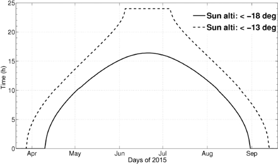
Fig. 2 Astronomical dark time at Dome A in 2015 calculated for the Sun's altitude of −18° (solid line) and −13° (dashed line).
Download figure:
Standard imageThe sky background contributed by moonlight depends on the Moon's position in the sky and lunar phase. Since the 18.6 year lunar nodal cycle changes the yearly declination range of the Moon, the Moon can reach a maximum altitude between ∼ 33° and ∼ 43° at Dome C (Kenyon & Storey 2006). Following the model by Krisciunas & Schaefer (1991), Kenyon & Storey (2006) calculated the moonlight brightness at Dome C and Mauna Kea in 2005. Their results indicate that the sky brightness contributed by moonlight increases gradually towards the Moon and then increases very sharply within 10° from the Moon. The sky would be brightened at zenith by moonlight by a median value of 1.7 mag arcsec−2 at Dome C in the V band between 2005 − 2015.
The Moon'smaximum altitude varies between ∼27° and ∼37° at Dome A, which is lower than at Dome C. The highest altitude of the Moon is ∼ 28° in 2015 (see Fig. 1). If we limit the zenith angle of the survey fields to be within 30° during Moon nights, the closest distance to the Moon would be 28°, which is much larger than 10°, and we can easily avoid the worst sky background. We have also estimated the moonlight contribution to the sky background using the same model (Krisciunas & Schaefer 1991) for Dome A. When the full Moon is at its highest altitude of 28° in 2015, which is the worst case at Dome A, the sky would be brightened by 1.2mag arcsec−2 in the i band at zenith (Fig. 3).

Fig. 3 Model sky brightness during a full Moon night when the Moon is at the highest altitude in 2015 at Dome A. The sky brightness is in magnitude per square arcsec, coded by color. The cross indicates the position of the Moon, and colored dots show the fields of the SN survey.
Download figure:
Standard imageAntarctica is different from temperate sites for optical astronomy because of aurorae. Aurorae are generally confined to an annular region between 15° and 25° from the geomagnetic South Pole, which is called the "auroral oval." The South Pole or Dome F lies close to the inner edge of the auroral oval, so they suffer from aurorae frequently. However, Dome A or Dome C lies only 6° from the geomagnetic South Pole, so aurorae lie below the horizon most of the time (Burton 2010; Kenyon & Storey 2006).
Since aurorae are caused by solar activities and are not predictable in practice, the scheduler does not take into account how to avoid aurorae. However, if future data allow us to study and figure out any regular patterns in location and time of aurorae, we will be able to optimize the scheduler accordingly.Currently, a practical and better way of avoiding aurorae is to design customized filters to exclude strong auroral emission lines.
4.1.2. Airmass and Extinction
As with any astronomical observations, we should try to minimize the atmospheric extinction when possible. For a large surveywith lots of fields, we can always set an upper limit on the zenith angle when selecting an optimal field to observe. As the Earth rotates, fields with larger zenith angle and airmass that are otherwise excluded can also meet the criteria at some time and be covered. The upper limit of zenith angle is a parameter that can be customized in the AST3 scheduler. The default value is 30°, indicating that AST3 can survey the sky fields with a declination ≤ −50° based on the latitude of Dome A of about −80°.
4.1.3. Pointing Limits of the Hour Angle
AST3 has an equatorialmount. Although it has two physical limit blocks on the hour angle that act as limits to protect the telescope and avoid cable entanglement, it is still preferable for the telescope not to hit the limit blocks. Therefore we also set soft hour angle limits in the scheduler. The default values are ±177°, slightly smaller than the hardware limits. Unlike a telescope at a lower latitude site, AST3 is able to point to all RA directions except for the small hour angle limits. There needs to be a way to prevent the telescope from reaching hour angle limits frequently. This is related to movement of the telescope and will be discussed together in the next section.
4.2. Minimal Slew
In order to save observing time and reduce observing overhead, we always want to minimize the slew of the telescope during the survey. One principle in choosing the next target field is that the scheduler should select the nearest available field to the current telescope position. The AST3 CCD camera has a rectangular field of view of 5 k×10 k pixels with the long edge along the Dec direction. Therefore the shortest path between two adjacent fields is in the RA direction. When the survey starts for the very first time, it will follow the increasing RA direction, then after each pointing, the scheduler configuration file records and updates the direction and the coordinates of the previous pointing. The survey keeps going in the RA direction until it reaches one of the limits (survey area boundary, airmass limit or hour angle limits, etc.). Then the survey will move to the next nearest Dec and change direction in the RA. This helps to save a lot of observing time compared to a survey that always goes in one RA direction and slews back when reaching a limit.
4.3. Time-domain Scientific Driver
The AST3 survey focuses on time-domain astronomy, including SN survey and exoplanet search. Different scientific goals of the project require different cadences of observing. The scheduler should be able to accommodate all the needs for the surveys.
As described above in Section 3.1, the cadences of the SN fields can be set with different preset priorities. However, the cadence of a general field with no priority can vary season by season because the dark time varies day by day (see Fig. 2). In order to keep a relatively uniform cadence for general survey fields, a flag of "observed" is added to the list of survey fields. Only when all fields are flagged will the scheduler clear all the flags and start the next round. This ensures that all fields have a uniform coverage in time and avoids excess observation of some areas because of their positions.
5. Flow Chart of survey scheduling
Based on the analyses above, we have implemented AST3's survey scheduler (Fig. 4). The scheduler works with the survey system to implement the automatic survey. The survey system queries the scheduler before each new pointing to determine what to do next, and this process repeats until the survey is stopped manually. Whenever asked, the scheduler first reads the configuration file to load a set of parameters. Therefore, the configuration file can be updated between observations.

Fig. 4 Survey scheduling flow chart, including both the special and survey modes.
Download figure:
Standard image
Fig. 5 Simulation of the survey process over a 24 h period, expressed in equatorial coordinates. The colored dots show footprints of the survey and the color scale from black to red indicates the time sequence. The survey starts from point a and always follows the RA direction unless indicated by arrows when a limit is hit. See text for more detailed explanations.
Download figure:
Standard imageAs the survey is fully automatic, the scheduler is able to make decisions on system standby, calibration (flat field) observing and scientific observing based on the altitude of the Sun. When the Sun is high enough, e.g., above −6°, the scheduler will notify the survey system to put the telescope in standby mode. The survey system asks the scheduler regularly until the Sun is in the twilight period, e.g., between −6° and −13°, and the scheduler will then do the flat-field observation.When the Sun is below −13° and dark time starts, scientific observations will start.
Since the special mode has the highest priority, the scheduler will check the special file first:
- (1)If the special target list is empty, switch back to the survey mode;
- (2)If not, check which targets are available for observing, and carry out the observations and update the special target list;
- (3)If more than one target can be observed at a time, select the nearest one to observe;
- (4)If no special targets in the list can be observed at a time, switch back to the survey mode, and get the coordinates for the next pointing.
The telescope runs in survey mode most of the time and it works as follows:
- (1)Read the survey field list, acquire information on all the fields, which includes ID, RA, Dec, priority level, number of times being observed, flag of "observed" in current run, time stamp of last observation, time stamp of being in current priority level, exposure time, number of exposures, CCD readout mode, name of observing type, etc.
- (2)Check the fields with the highest priority level (i.e. n = 0) and update the priority according to preset priority rules. Carry out the observations if there are still fields with the highest priority level. Update the time stamps in the survey field list.
- (3)Repeat above for fields with lower priority levels.
- (4)When reaching fields with priority level of n = 6, i.e., the general field without a specified cadence, the scheduler operates as a normal survey:
- (a)Read in previous pointing position and survey direction of the normal survey.
- (b)Check whether the last field reaches any limit at the time. If so, select the field with the next Dec near the limit and change the survey direction in RA. If not, select the next field with the same Dec in the current survey direction in RA.
- (c)Update the survey field list with this position and direction, and mark the field as observed.
- (5)Output information on the selected field, including observing information (coordinates in equatorial system, exposure time, number of exposures in one imaging sequence, readout mode) and associated information (coordinates in the horizontal system, airmass, coordinates of Sun/Moon in the equatorial/horizontal system, phase of the Moon, angular distance between the target field and the Sun/Moon, etc.).
- (6)Make the survey system wait for the next call.
The survey mode includes both SN and exoplanet survey modes. The basic concepts for these two modes are the same except that the exoplanet mode does not need to worry about special targets or different priorities and is simpler. A parameter in the configuration file determines which mode is activated.
In order to demonstrate the survey process, we show a simple simulation which covers over 2400 square degrees of the southern sky in 24 h during the polar night (see Fig. 4). We select fields with RA between −50° and −70° and avoid the Galactic plane between Galactic latitudes of ±20°. The allowed hour angle range is between −177° and 177°. The survey starts at point a and moves towards point b along the same Dec. When it reaches the limit of the Galactic latitude at point b, the survey switches to the nearest Dec and turns around in the RA direction towards point c where it does the same due to the limit of hour angle. Label d indicates a long slew when all fields with positive hour angle have been observed and the telescope has to move to the other side of the meridian with minimal slew. This is the only long slew over a 24 h period. The arrow connecting cyan points near a and c indicates that all fields with Dec of −70° have been observed, so the survey moves to the next Dec but avoids observed fields.
6. Conclusions
We have developed a customized scheduler for the automatic AST3 survey at Dome A, Antarctica. By taking into account many factors that can affect the efficient use of observing time and data quality, the scheduler is able to select the best field for observing in real-time. It has been used with the AST3 survey system and proved to be very reliable. This work will also be useful for the future Kunlun Dark-Universe Survey Telescope (KDUST) or other sky surveys requiring real-time, automatic response of telescope operation.
Acknowledgements
This work has been supported by the Chinese Polar Environment Comprehensive Investigation & Assessment Programmes (Grant No. CHINARE2017-02-04), the National Natural Science Foundation of China (Grant Nos. 11003027, 11403057, 11403048, 11203039 and 11273019), and the National Basic Research Program of China (973 Program, Grant No. 2013CB834900).