Effects of frequency-dependent membrane capacitance on neural excitability

We modeled a frequency-dependent capacitance, c(s), using the following expression:

$$\begin{eqnarray}&&c(s)={c}_{\infty }+\displaystyle \frac{{c}_{{\rm{\Delta }}}}{1+s\tau },\end{eqnarray} \tag{ 1 }$$

$$\begin{eqnarray}&&{c}_{{\rm{\Delta }}}={c}_{{\rm{dc}}}-{c}_{\infty },\end{eqnarray} \tag{ 2 }$$

$$\begin{eqnarray}&&s=j\omega ,\end{eqnarray} \tag{ 3 }$$

where, c_dc is the specific membrane capacitance (F m⁻²) at ω = 0; c_∞ is the membrane capacitance at ω = ∞; τ is the relaxation time (s); and ω = 2πf is the angular frequency (rad s⁻¹).

The impedance of c(s) (in Ω m⁻²) is given by equations (4), and (5) is the ordinary differential equation (ODE) that describes the relationship between the capacitive current density (i_c in A m⁻²) and the transmembrane voltage (V_m) across the capacitor

$$\begin{eqnarray}&&{z}_{c}=\displaystyle \frac{1}{sc(s)},\end{eqnarray} \tag{ 4 }$$

$$\begin{eqnarray}&&{b}_{1}{V^{\prime\prime} }_{m}+{b}_{0}{V^{\prime} }_{m}={a}_{1}{i^{\prime} }_{c}+{a}_{0}{i}_{c}.\end{eqnarray} \tag{ 5 }$$

The prime symbol denotes the derivative with respect to time; and a₀ = 1, a₁ = τ, b₀ = c_dc, and b₁ = τc_∞ are constant coefficients determined with equation (1).We reduced equation (5) to a system of first order ODEs. However, preliminary analysis showed that this system of ODEs was moderately stiff (see appendix) and thereby presented issues for numerical solution.

We therefore used a combination of linear circuit elements to model the frequency dependent capacitance, c(f) (figure 1). The circuit representing c(f) consisted of a capacitance (c_∞) in parallel with the series combination of a conductance (g_Δ in S m⁻²) and capacitance (c_Δ), and had an impedance equal to that of equation (4). The ODEs describing the relationship between V_m and i_c are given in the appendix.

Zoom In Zoom Out Reset image size

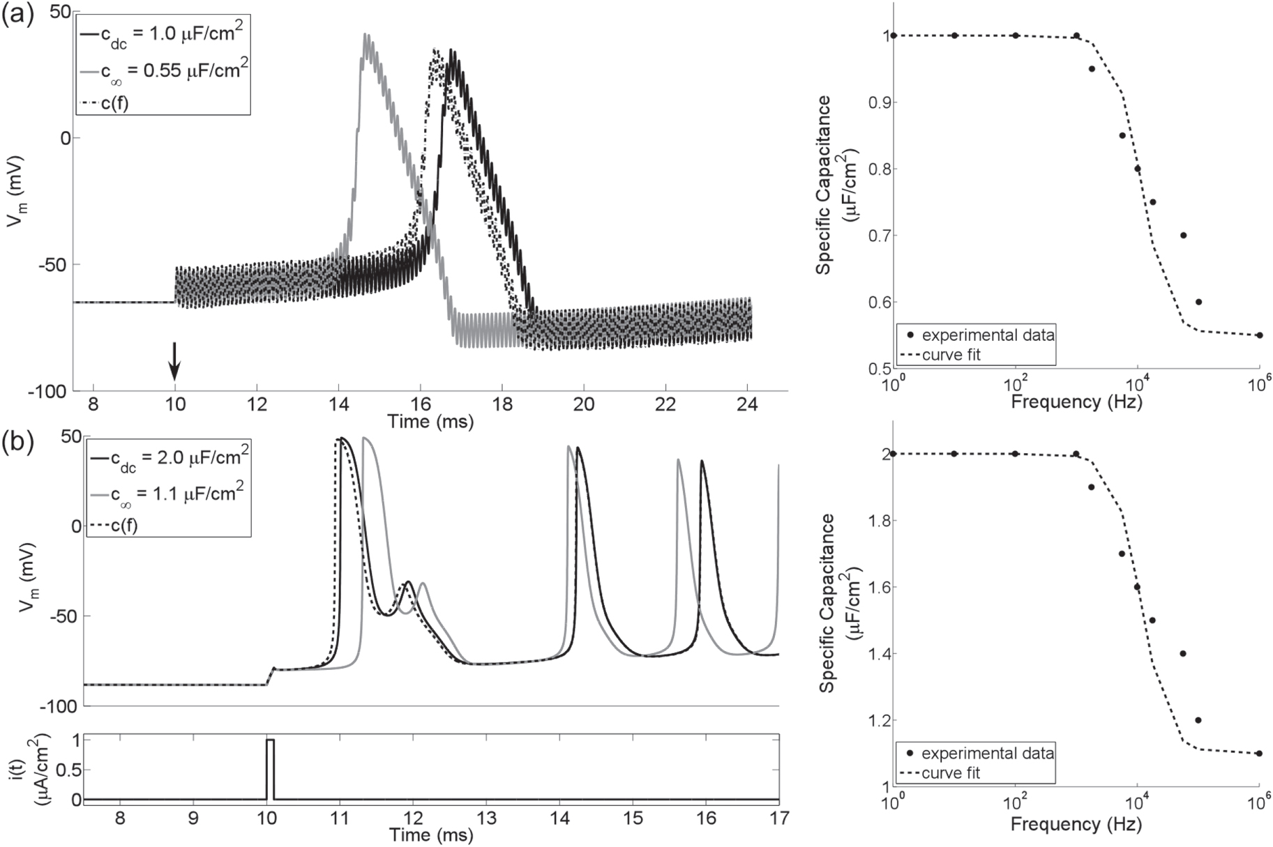
We implemented two single-compartment lumped models (SCMs) of neurons in MATLAB (v2014a, Mathworks, Natick, MA). The first, HH SCM, included Hodgkin–Huxley (HH) ion channels (Hodgkin and Huxley 1952) and either a constant membrane capacitance or c(f). The constant membrane capacitance was set to either c_dc = 1 μF cm⁻² or c_∞ = 0.55 μF cm⁻², while c(f) declined from c_dc to c_∞ with τ = (2π10⁴)⁻¹ s (figure 2(a)). We selected values for c_dc, c_∞, and τ based on measurements from a squid giant axon (Takashima and Schwan 1974).

Zoom In Zoom Out Reset image size

The second, MRG SCM, included ion channels representative of mammalian nerve fibers (McIntyre et al 2002) and either a constant membrane capacitance or c(f). We set c_dc = 2 μF cm⁻² (Frankenhaeuser and Huxley 1964), as there are no studies that analyze how the membrane capacitance varies with frequency in mammalian axons. c_∞ was set to 1.1 μF cm⁻², and τ was kept at (2π10⁴)⁻¹ s.

A more detailed description of the ODEs and parameters of the HH and MRG SCMs is given in the appendix.

2.2.1. Lumped model validation, and implementation, and analysis

We used a linear circuit representation of the neural membrane (figure 1(b)) to validate the numerical solutions of the SCMs. The solution was approximated using the stiff ordinary different equation solver, ode15s, in MATLAB, and we verified that the root mean square error between the numerical and analytical solutions was <5 × 10⁻⁴ % (see appendix).

We used three different types of intracellular current waveforms (A m⁻²) to stimulate the SCMs: a monophasic rectangular pulse, a train of monophasic rectangular pulses, and a sine wave (figure 3). The pulse widths (PWs) of monophasic rectangular pulses ranged from 50 μs to 10 ms, as this range encompasses the range of possible PWs used in electrical stimulation devices.

Zoom In Zoom Out Reset image size

For stimulation with a train of pulses, PW was set to 100 μs, a typical PW used in deep brain stimulation (Kuncel and Grill 2004), and the frequency of the pulse train ranged from 100 Hz to 10 kHz. Below 100 Hz, the stimulation thresholds were identical to the stimulation thresholds with a single pulse, and at and above 10 kHz, the pulses fused to produce direct-current stimulation. Therefore, only stimulation thresholds within the above range were analyzed.

For sinusoidal stimulation currents, frequencies ranged between 100 Hz and 100 kHz. The lower bound of this range was chosen because we assumed that no dispersion occurred at frequencies below 100 Hz (see section 4.3), and the upper bound was chosen so that it encompassed the frequencies used in vivo for studying conduction block (Bhadra and Kilgore 2005, Joseph and Butera 2009).

The nonlinear SCMs (figure 1(a)) were solved using ode15 s. For stimulation with rectangular pulses, we used a variable time-step with a maximum step of 10 μs for PWs ≥100 μs, and 5 μs for PWs <100 μs; and for sinusoidal stimulation, we used a variable time-step with a maximum of 10 ns for frequencies below 10 kHz and 0.5 ns for frequencies above 10 kHz. In all simulations, reducing the maximum time-steps by half altered the stimulation thresholds by <1%. Further, we imposed a 10 ms delay to ensure the model had reached steady-state before stimulation, and all simulations were run for 30 ms.

Thresholds to generate an action potential were calculated using a bisection algorithm (relative error <1%), and traces of V_m were inspected post hoc to ensure that at least one action potential was evoked at the calculated value (figure 2).

We implemented two distributed models of axons in NEURON (v7.3) (Carnevale and Hines 1997): a HH model of an unmyelinated axon with the same ion channels used in the HH SCM and an (McIntyre–Richardson–Grill) MRG model of a myelinated axon, which, at the nodes of Ranvier, contained the same ion channels used in the MRG SCM. The values that defined the membrane capacitance in the HH axon and MRG axon were the same as those used in the HH SCM and MRG SCM, respectively (see section 2.2). For the unmyelinated fiber model, we used a 40 mm long axon segmented in 0.5 mm long cylinders (Tai et al 2005), and the axons had diameters ranging from 50 to 800 μm to represent the squid giant axon (Matsumoto and Tasaki 1977), and from 0.4 to 2 μm to represent mammalian unmyelinated axons. The myelinated axons were at least 10 mm in length and had diameters (including the myelin) ranging from 5.7 to 16 μm. The geometric and electric parameters of the myelin and intermodal regions were taken from a validated model of a mammalian myelinated axon (McIntyre et al 2002). Both the myelinated and unmyelinated axons were long enough to avoid activation at the terminations of the axons, and we confirmed that in all of our simulations no action potentials were generated at the ends.

2.3.1. Distributed model implementation and analysis

A number of analyses were conducted to assess the effects of c(f) on neural excitability: (1) stimulation thresholds (see section 2.2.2); (2) the recovery cycle, which is the change in stimulation thresholds following a supra-threshold conditioning stimulus; (3) the strength–distance relationship, which is the relationship between the stimulation thresholds and the axon-to-electrode distance; (4) the firing rate of the axon during repetitive pulse stimulation; (5) thresholds for conduction block; and (6) conduction velocity.

Stimuli were extracellular currents delivered in an infinite medium with homogeneous and anisotropic conductivity. The longitudinal (σ_z) and transverse (σ_xy) conductivity were 1/3 and 1/12 S m⁻¹, respectively (McIntyre et al 2002). We calculated the extracellular potentials using the following function (Li and Uren 1998):

$$\begin{eqnarray}&&{\rm{\Phi }}(x,y,z)=\displaystyle \frac{{I}_{s}}{4\pi \sqrt{{\sigma }_{xy}{\sigma }_{z}({x}^{2}+{y}^{2})+{\sigma }_{xy}^{2}{z}^{2}}},\end{eqnarray} \tag{ 6 }$$

where, I_s is the amplitude of a point source current (in A), which was located at the origin; and x, y, and z are the coordinates of a point on an axon. We calculated the extracellular potentials in MATLAB and used the 'extracellular' mechanism in NEURON to apply extracellular stimulation to the model axons. We implemented c(f) in NEURON by setting the membrane capacitance equal to zero and using the 'LinearMechanism' class to define the corresponding ODEs (see appendix). The axon models were solved using an implicit (trapezoidal) integration method with a fixed time step of 1 μs. Halving the time step altered the stimulation thresholds by <1%. Unless stated otherwise, there was a 1 ms delay before the onset of stimulation, and all simulation were run for a total of 10 ms.

To analyze the recovery cycle, we stimulated a 5.7 μm diameter axon at an electrode-to-axon distance of 0.6 mm. The point source electrode was positioned over the middle node of Ranvier. The output metric was the percent difference in the stimulation threshold between two 1 ms rectangular pulses over inter-pulse intervals between 2.5 and 100 ms, as axons fully recover excitability after 100 ms (Kiernan et al 1996).

In the strength–distance analysis, we stimulated a population of fifty myelinated axons with diameters of 5.7 μm, and each simulation was independent of each other, i.e., there were no axon–axon interactions. The axons were randomly placed in the medium so that the electrode-to-axon distances (r) were uniformly distributed between 0.1 and 1 mm—a range in which thresholds have been measured experimentally (BeMent and Ranck 1969)—and the central node of Ranvier was laterally displaced by between −0.5 and +0.5 inter-nodal lengths from the point source electrode. We used least-squares regression to fit the stimulation thresholds (I_th) to the function: I_th = k₁ + k₂r², where k₁ and k₂ are constant coefficients. The output metric in this analysis was k₂.

To quantify the response of the distributed fiber models to repetitive pulse stimulation, we applied a train of 50 rectangular pulses of 100 μs duration and amplitude 10% larger than the threshold for a single pulse. The time between the pulses ranged from 0.1 to 10 ms (i.e., frequencies of 100 Hz to 10 kHz), and the duration of the simulation was set to deliver 50 pulses. We counted the number of action potentials to obtain the spikes per pulse, which was the output metric in this analysis.

To quantify thresholds to achieve block of action potential conduction, we followed the approach of (Bhadra et al 2007). Using an extracellular point source electrode located 1 mm above the middle of the fiber, we delivered a sinusoidal signal (3–40 kHz). 40 ms after the onset of the sinusoidal signal, we applied an intracellular test stimulus to one end of the fiber and determined whether the evoked action potential propagated to the other end. We used a bisection algorithm (1 μA resolution) to determine the minimum amplitude of the extracellular sinusoidal signal that blocked the conduction of the test action potential.

Finally, the conduction velocity was calculated by applying a suprathreshold 250 μs rectangular stimulus to a 101-node fiber and averaging local conduction velocities from node to node for the myelinated fiber and in segments of 0.5 mm for the unmyelinated fiber. Displacements from the location where the action potential was initiated to the location where the action potential was recorded were positive; therefore, by definition, all velocities were positive.

We quantified the effect of c(f) on the firing rate of a model of a pyramidal neuron from prefrontal cortex (PFC). We used the 'intrinsic bursting' cell type of (Sidiropoulou and Poirazi 2012), and the NEURON implementation as available in the modelDB database (https://senselab.med.yale.edu/modeldb/ShowModel.asp?model=144089). The model comprises a large variety of membrane mechanisms distributed in one axon, one soma and 43 dendrites, and includes an artificial current with Poisson characteristics to simulate the ion channel noise observed in vitro. We inserted c(f) in all compartments as described in section 2.3.1. We applied intracellular 500 ms constant current stimulation to the soma and quantified the number of action potentials. We calculated the input-output response function, i.e., the f–I curve, defined as the average firing rate as a function of stimulus amplitude in the range from 0.1 to 1.6 nA. Next, we applied natural patterns of synaptic stimulation as described in detail in (Sidiropoulou and Poirazi 2012). Briefly, the dendrites were stimulated with 200 randomly distributed excitatory synapses that were activated 10 times at 20 Hz, and the soma was stimulated with 5 inhibitory synapses at 50 Hz. In this test, we increased the conductance of the Ca⁺⁺-activated non-selective cation (CAN) current to 106 μS cm⁻² to induce persistent activity and calculated the inter-spike interval (ISI) distribution for 25 five s duration simulations that differed in the randomly selected location of the excitatory synapses.

The effects of c(f) on thresholds for stimulation and block depended on the ion-channel kinetics and stimulation waveform. c(f) had a negligible effect on the stimulation thresholds of SCM neurons with HH ion channels: across all cases, stimulation thresholds were altered by at most 6.3% (median = 1.4%). In contrast, c(f) had a marked effect on the stimulation thresholds of the MRG SCM but only for sinusoidal waveforms (figure 3). In the MRG SCM, incorporation of c(f) decreased the stimulation thresholds of sinusoidal waveforms by up to 48% at f > 8 kHz. However, changing from c_dc to c(f) had negligible impact on the stimulation thresholds with a train of 100 μs pulses at frequencies between 100 Hz and 10 kHz.

Similar results were observed in the distributed axons models, and the effect was slightly more accentuated in smaller diameter fibers (figure 4(c)). The activation thresholds using sinusoidal stimulation declined by up to 19.3%, 14% and 11.5% for MRG axons with fiber diameters of 5.7, 11.5 and 16 μm, respectively. For unmyelinated axons, the activation thresholds varied less than 5.6% (median = 0.2%). The fidelity of the fiber response to repetitive pulsatile stimulation, which deteriorated at shorter inter-pulse intervals, was not affected by c(f) (figure 4(d)).

Zoom In Zoom Out Reset image size

c(f) had negligible effects on both the recovery cycle and strength–distance relationship of the axon models (figure 4). Switching from c_dc to c(f) altered the recovery cycle by at most 1.4% (median = 0.4%) and k₂ by 7.9 %. In the strength–distance relationship, the lateral displacements of the nodes relative to the electrode affected the thresholds, and this effect was greater for shorter electrode-to-axon distances. The thresholds were more widely scattered for electrode-to-axon distances smaller than 0.5 mm, and the subset of axons laterally displaced by less than 0.1 inter-nodal lengths had thresholds ∼60% lower than those displaced more than 0.3 inter-nodal lengths (figure 4(b)). On the other hand, this difference decreased to ∼10% for electrode-to-axon distances greater than 0.5 mm. This was expected because fiber excitation with monopolar point-source electrodes is more affected by the distance from the electrode to the closest node than the perpendicular distance to the fiber (Rattay 1989).

3.1.1. Thresholds for conduction block with sinusoidal signals

The threshold amplitudes of a sinusoidal signal to achieve block of action potential conduction were reduced by c(f), and the effect was more pronounced for smaller diameter fibers and higher signal frequencies (figure 5). The maximum reductions in block threshold were 11.5% (median 5.7%), 5.9% (median 3%) and 5.5% (median 1.8%) for fiber diameters of 5.7, 10 and 15 μm, respectively.

Zoom In Zoom Out Reset image size

The action potential conduction velocity was increased by the incorporation of c(f), and the effect was greater for the myelinated fiber (figure 6). The maximum increase in conduction velocity was 7.9% (median 7.1%) and 1.7% (median 1.3%) for the myelinated and unmyelinated fibers, respectively.

Zoom In Zoom Out Reset image size

The incorporation of c(f) had a minimal effect on the firing properties of the model of a PFC neuron. Although reducing the (constant) capacitance to c_∞ increased the firing rate by up to 25%, the f–I curve with c(f) overlapped with that with c_dc (figure 7(b)). With the simulated natural patterns of excitation, the model neuron fired persistently for both the c_dc and the c(f) cases, but fired slightly more rapidly in the latter case, as reflected in the ISI histogram (figure 7(c)). The median ISI for c_dc and c(f) was 15.9 ms (min = 0.2, max = 106.2) and 15.7 ms (min = 0.2, max = 84.2), respectively, across 25 simulations.

Zoom In Zoom Out Reset image size

The decrease in the membrane capacitance with increasing frequency, or dielectric dispersion, can be modeled as an $n-{\rm step}$ relaxation process (Awayda et al 1999):

$$\begin{eqnarray}&&c(s)={c}_{\infty }+\displaystyle \sum _{i=1}^{n}\;\displaystyle \frac{{c}_{{\rm{\Delta }},i}}{1+{(s{\tau }_{i})}^{{\gamma }_{i}}},\end{eqnarray} \tag{ 7 }$$

$$\begin{eqnarray}&&{c}_{dc}-{c}_{\infty }=\displaystyle \sum _{i=1}^{n}\;{c}_{{\rm{\Delta }},i},\end{eqnarray} \tag{ 8 }$$

where, for the ith relaxation step, c_Δ,i is the change in the membrane capacitance, τ_i is the relaxation time, and γ_i is the Cole–Cole power-law factor, which is between 0 and 1 (Cole and Cole 1941, Cole and Cole 1942). In our analyses, we approximated dielectric dispersion using one relaxation step (i.e., n = 1), and we assumed γ₁ = γ = 1 so that c(f) could be modeled using linear circuit elements.

Dielectric dispersion at frequencies below 100 kHz is typically referred to as α dispersion and is associated with ionic diffusion processes at the cell membrane (Foster and Schwan 1989). Because the relaxation event occurring at the neural membrane is not a first order process (Chew and Sen 1982), one τ may not be suitable to describe α dispersion. The representation of c(f) can be improved by using n + 1 capacitances and n conductances to model n relaxation steps (figure 8(a)). For example, using two relaxation steps better approximated the experimental values of c(f) (figure 8(b)), but despite the better fit to the data, the stimulation thresholds only changed by at most 8.3% (median = 2.0%) compared to n = 1 (figure 8(c)). Therefore, one τ was a reasonable approximation for α dispersion.

Zoom In Zoom Out Reset image size

Alternatively, the assumption that all τ_i are all well separated (i.e., τ₁ ≪ τ₂ ≪ ... ≪ τ_n) can be relaxed, which means some γ_i ≠ 1 (Foster and Schwan 1989). For many biological tissues, γ_i ≠ 1 (Gabriel et al 1996c); therefore, the γ_i that describe dispersion in the neural membrane are likely not equal to one. For n = 1, changing γ from 1 to 0.7 reduced the relative percent difference between c(f) and the experimental data (figure 2(a)) from between −19% and +7.3% (figure 2(a)) to between −10% and +4.3% at frequencies between 1 kHz 100 kHz (not shown). However, relaxing the assumption that all γ_i = 1 is not trivial because this leads to a relationship between V_m and i_c that involves fractional derivatives (Biswas et al 2006). Solving a system of ODEs with fractional derivatives is not as straightforward as solving a system of ODEs with integer-valued derivatives (Diethelm et al 2005). Therefore, it may be more practical to use a larger n with all γ_i = 1 than a smaller number of n with 0 < γ_i < 1, as the former may be more computationally tractable.

4.2.1. The effects on stimulation thresholds

To understand why c(f) had an effect in some instances but not in others, we must first understand how changing a constant membrane capacitance (c_m) affects V_m. For a constant c_m, ${i}_{c}={c}_{m}{V^{\prime} }_{m},$ and

$$\begin{eqnarray}&&{V}_{m}(t)={c}_{m}^{-1}\displaystyle {\int }_{0}^{t}{i}_{c}(u){\rm{d}}u.\end{eqnarray} \tag{ 9 }$$

As positive and negative charge builds up on the inner and outer surfaces of the neural membrane, respectively, the membrane is depolarized, and V_m increases more for a membrane with a smaller c_m. In other words, when c_m is smaller, it takes less charge to reach the threshold for excitation. This explains why decreasing c_m from c_dc to c_∞ decreased stimulation thresholds (figure 3).

Next, we consider how the spectrum of V_m affects c(f). Below the threshold for excitation, the response of the neural membrane to a rectangular pulse of intracellular current resembles the response of the parallel combination of a resistor and capacitor (figure 9(a)). Since the majority of the signal power in this exponential response is in the frequency band below 1 kHz (figure 9(a)), and since c(f) ≈ c_dc for frequencies <1 kHz, one expects that pulse stimulation thresholds will not be markedly different between the c(f) and c_dc cases (figures 3(a) and (c)).

Zoom In Zoom Out Reset image size

With a train of rectangular pulses, the majority of the power in V_m is also in the frequency band below 1 kHz, even if the pulses are delivered at frequencies greater than 1 kHz. For example, consider a train of 100 μs pulses delivered at 5 kHz. One expects that V_m will have spectral content at 5 kHz because the power-spectral density of a 5 kHz train of pulses is maximal at the stimulation frequency. Indeed, during subthreshold stimulation, V_m appears to oscillate at 5 kHz but about a dynamic baseline that resembles the response of the parallel combination of a resistor and capacitor to a direct-current stimulus (figure 9(b)). This occurs because as the frequency of the train approaches its fusion frequency (10 kHz, in this example), more power is concentrated near 0 Hz (figure 9(b)), explaining why the stimulation thresholds did not differ markedly between the c(f) and c_dc cases.

Unlike the pulsed rectangular stimulation, V_m followed the frequency of stimulation during subthreshold sinusoidal stimulation, and the majority of the power in the membrane response was concentrated near the stimulation frequency (figure 9(c)). Therefore, at stimulation frequencies where c(f) was substantially less than c_dc, one expects a reduction in the stimulation thresholds, which is what was observed (figure 3(b)).

Examination of V_m also explained why c(f) had an effect on the MRG model thresholds but not on the HH model thresholds. At the onset of the sinusoidal stimulus, V_m oscillated at the stimulation frequency about a transiently changing baseline, which is known as the natural or characteristic response of the system. The time constant of the natural response (τ_nat) is equal to c_m/g_m, which is approximately equal to c_m/g_L for sub-threshold stimulation. Because g_L in the HH model was more than 10 times larger than g_L in the MRG model (see appendix), the natural response was significantly longer in the HH model (figure 10(a)). In the HH models, the natural response exhibited a marked amount of signal power in the frequency band below 1 kHz (figure 10(a)), which, we hypothesized, caused c(f) to behave more like c_dc.

Zoom In Zoom Out Reset image size

If the natural response was the reason that c(f) had a negligible effect on sinusoidal stimulation thresholds in the HH models, then reducing the magnitude of the natural response should alter the results. We tested this prediction using a modified sinusoidal stimulus: the peak-to-peak amplitude of the sinusoid increased linearly from 0 to its maximum value over the course of 1 ms (figure 10(b)), and this substantially reduced the magnitude of the natural response. With the ramped sinusoid, stimulation thresholds decreased appreciably for frequencies >10 kHz (figure 10(c)), which is what was observed in the MRG model (figure 3(b)).

Moreover, we calculated the frequency response of the equivalent circuit proposed by (Sabah and Leibovic 1969) for small-signal approximation of an HH cell (figure 10(d)). The admittance, Y, of this circuit quantifies the steady-state transmembrane voltage for a sub-threshold sinusoidal current stimulus. The magnitude of Y increased with increasing frequency similarly to the threshold for sinusoidal stimulation, and upon incorporation of c(f), Y deviated for frequencies >1 kHz. This further supports the effect of the natural response on the HH cell, since the admittance does not account for the transient cell response. Therefore, the natural response could explain the qualitative differences in the sensitivity of the HH and MRG models to the representation of the membrane capacitance.

4.2.2. The effects on the thresholds for conduction block

4.2.3. The effects on conduction velocity

4.2.4. The effects on firing rate

We limited our analysis to three basic waveforms: a monophasic rectangular pulse, a train of monophasic rectangular pulses, and a sinusoid. Simplifying the stimuli allowed us to develop a fundamental understanding of how c(f) affected neural excitability. However, in practice, the waveforms used for electrical stimulation are more complex. For example, the rectangular waveforms used in electrical stimulation therapies typically have two phases; the first (stimulation) phase is used to elicit the physiological response, and the second (opposite polarity charge-balancing) phase is used to reverse electrochemical reactions that may damage the electrode and/or tissue (Merrill et al 2005).

To determine if a charge-balancing phase would alter the conclusions, we used a biphasic rectangular pulse to stimulate the MRG SCM. At all the PWs considered in this study (i.e., 50 μs to 10 ms), the addition of a symmetric charge-balancing phase of equal duration altered the stimulation thresholds by at most 7.9% (median = 0%) when the membrane capacitance was changed from c_dc to c(f). The charge-balancing phase in many electrical stimulation therapies, however, is not symmetric but asymmetric. Similar results were observed when the charge-balancing phase was 9 times the duration and 1/9 times the amplitude of the stimulation phase. Therefore, we predict that the trends observed in this study will not be greatly impacted by the addition of a subsequent charge-balancing phase.

However, there are other aspects of electrical stimulation that may also play a role in altering the shape of the stimulation waveform. For example, the charge transduction process that occurs at the electrode–tissue interface (ETI) (Butson and McIntyre 2005, Cantrell et al 2008, Howell et al 2014) and dielectric dispersion in the nervous tissue (Bossetti et al 2008, Medina and Grill 2014) can both alter the time course (shape) of the voltages appearing in the tissue. We observed that modification to the stimulus waveform could alter the response of the neural membrane and thereby the effects c(f) on neural excitation (figure 10). Therefore, when studying the effects of c(f) in specific applications of electrical stimulation, the charging of the ETI and dielectric dispersion in the tissue should also be considered.

The parameterization of c(f) in this study was based on data from a limited number of studies on squid giant axons (Takashima and Schwan 1974, Haydon et al 1980, Haydon and Urban 1985). These studies all indicate that the membrane capacitance is approximately constant from 100 Hz to 1 kHz and declines by approximately 50% between 1 and 100 kHz. Because none of these studies provided data for frequencies below 100 Hz, we assumed the low frequency membrane capacitance was constant. We also assumed that the membrane capacitances of mammalian and squid axons would exhibit similar frequency dependence. These were reasonable assumptions given the goal of this study was to develop an understanding of how c(f) impacted neural excitability.

We modeled a lumped single-compartment (SCM) neuron with linear circuit elements representing the neural membrane (figure 1(b)). The membrane conductance (g_m in S m⁻²) was constant and the membrane capacitance varied with frequency. The following system of ODEs model the response of the SCM neuron to a single monophasic rectangular pulse:

$$\begin{eqnarray}&&\bar{v}^{\prime} =A\bar{v}+\bar{b},\end{eqnarray} \tag{ A.1 }$$

$$\begin{eqnarray}\bar{v}={[\begin{array}{cc}{V}_{m} & {V}_{c{\rm{\Delta }}}\end{array}]}^{T},\end{eqnarray} \tag{ A.2 }$$

$$\begin{eqnarray}A=[\begin{array}{cc}{a}_{11} & {a}_{12}\\ {a}_{21} & {a}_{22}\end{array}]=[\begin{array}{cc}-{c}_{\infty }^{-1}\{{g}_{{\rm{\Delta }}}+{g}_{m}\} & {c}_{\infty }^{-1}{g}_{{\rm{\Delta }}}\\ {c}_{{\rm{\Delta }}}^{-1}{g}_{{\rm{\Delta }}} & -{c}_{{\rm{\Delta }}}^{-1}{g}_{{\rm{\Delta }}}\end{array}],\end{eqnarray} \tag{ A.3 }$$

$$\begin{eqnarray}\bar{b}={[\begin{array}{cc}{c}_{\infty }^{-1}({i}_{s}(t)+{V}_{{\rm{rest}}}{g}_{m}) & 0\end{array}]}^{T}.\end{eqnarray} \tag{ A.4 }$$

The frequency-dependent membrane capacitance consisted of a capacitance (c_∞) in parallel with the series combination of a conductance (g_Δ) and capacitance (c_Δ). V_m and V_rest denote the transmembrane and rest voltages, respectively; V_cΔ is the voltage drop across c_Δ; i_s(t) is the waveform of the applied stimulus (in A m⁻²); the bar denotes a vector quantity; and T is the transpose operator.

When i_s(t) is a single monophasic rectangular pulse, the solution of equations (A.1)–(A.4) takes the following form:

$$\begin{eqnarray}&&v={k}_{1}exp({\lambda }_{1}t){\bar{u}}_{1}+{k}_{2}{\rm exp}({\lambda }_{2}t){\bar{u}}_{2}+\bar{f},\end{eqnarray} \tag{ A.5 }$$

$$\begin{eqnarray}U=[\begin{array}{cc}{\bar{u}}_{1} & {\bar{u}}_{2}\end{array}],\end{eqnarray} \tag{ A.6 }$$

$$\begin{eqnarray}\bar{k}={[\begin{array}{cc}{k}_{1} & {k}_{2}\end{array}]}^{T},\end{eqnarray} \tag{ A.7 }$$

$$\begin{eqnarray}&&\bar{f}={A}^{-1}\bar{b},\end{eqnarray} \tag{ A.8 }$$

$$\begin{eqnarray}\bar{k}={U}^{-1}({[\begin{array}{cc}{V}_{o} & {V}_{o}\end{array}]}^{T}-\bar{f}).\end{eqnarray} \tag{ A.9 }$$

λ_1/2 are the eigenvalues of (A.3), and V_o is the initial value of V_m. We compared the analytical solution (i.e., (A.5)–(A.9)) to the numerical solution (see section 2.1.1). The root mean square error (RMSE) between the numerical and analytical solutions was <5 × 10⁻⁴%.

When i_s(t) is a sinusoid, the solution of equations (A.1)–(A.4) takes the following form:

$$\begin{eqnarray}&&\bar{v}={k}_{1}exp({\lambda }_{1}t){\bar{u}}_{1}+{k}_{2}{\rm exp}({\lambda }_{2}t){\bar{u}}_{2}\\ \quad \;\;\;\;\;+H{[\begin{array}{ccc}{\rm cos}(\omega t) & {\rm sin}(\omega t) & 1\end{array}]}^{T},\end{eqnarray} \tag{ A.10 }$$

$$\begin{eqnarray}H=[\begin{array}{c}\begin{array}{ccc}{h}_{12} & {h}_{12} & {h}_{13}\end{array}\\ \begin{array}{ccc}{h}_{21} & {h}_{22} & {h}_{23}\end{array}\end{array}],\end{eqnarray} \tag{ A.11 }$$

$$\begin{eqnarray}\bar{h}={[\begin{array}{cc}\begin{array}{ccc}{h}_{11} & {h}_{12} & {h}_{13}\end{array} & \begin{array}{ccc}{h}_{21} & {h}_{22} & {h}_{23}\end{array}\end{array}]}^{T}\\ \quad ={L}^{-1}[\begin{array}{cc}\begin{array}{ccc}0 & {c}_{\infty }^{-1}{I}_{s} & {c}_{\infty }^{-1}{V}_{{\rm{rest}}}{r}_{m}^{-1}\end{array} & \begin{array}{ccc}0 & 0 & 0\end{array}\end{array}],\end{eqnarray} \tag{ A.12 }$$

$$\begin{eqnarray}L=[\begin{array}{cccccc}-{a}_{11} & \omega & 0 & -{a}_{12} & 0 & 0\\ -\omega & -{a}_{11} & 0 & 0 & -{a}_{12} & 0\\ 0 & 0 & {a}_{11} & 0 & 0 & {a}_{12}\\ -{a}_{21} & 0 & 0 & -{a}_{22} & \omega & 0\\ 0 & -{a}_{21} & 0 & -\omega & -{a}_{22} & 0\\ 0 & 0 & {a}_{21} & 0 & 0 & {a}_{22}\end{array}],\end{eqnarray} \tag{ A.13 }$$

$$\begin{eqnarray}\bar{k} & = & [\begin{array}{cc}{k}_{1} & {k}_{2}\end{array}]\\ & = & {U}^{-1}{([\begin{array}{cc}{V}_{o} & {V}_{o}\end{array}]-[\begin{array}{cc}{h}_{11}+{h}_{13} & {h}_{21}+{h}_{23}\end{array}])}^{T}.\end{eqnarray} \tag{ A.14 }$$

For sinusoidal stimulation, the RMSE between the numerical and analytical solutions (A.10)–(A.14) was <5 × 10⁻⁴%.

We used the ratio of the largest eigenvalue to the smallest eigenvalue, known as the stiffness ratio (LeVeque 2007),

$$\begin{eqnarray}&&S=\displaystyle \frac{{\rm{max}}(|{\lambda }_{i}|)}{{\rm{min}}(|{\lambda }_{i}|)}\in i=1,\;2\end{eqnarray} \tag{ A.15 }$$

to assess the numerical stability of the ODEs describing c(f). || denotes the absolute value or magnitude of the eigenvalues. If a system of ODEs is stiff, S is typically ≫1, which means small to moderate perturbations in the system can lead to large fluctuations in some variables that force the numerical method to have large errors or become unstable (Spijker 1996). For (A.3), S ≈ 230.

When c(f) was modeled using equation (5), achieving an RMSE of <5 × 10⁻⁴ between the analytical and numerical solution required time step sizes of <0.5 μs. To compare, when c(f) was modeled using equations (A.1)–(A.4), achieving the same degree of accuracy required time step sizes of <0.1 ms. Compared to the other variables, the values of ${i^{\prime} }_{c}$ (see equation (5)) were disproportionately large, which could explain the large errors that resulted when modeling c(f) with equation (5). Therefore, the stiffness of the ODEs consider in this work was only an issue when dealing with higher order terms (e.g., ${i^{\prime} }_{c},$ ${V^{\prime\prime} }_{m}$).

We used the equations from the seminal work of Hodgkin and Huxley to model three current densities in a SCM of a HH neuron (Hodgkin and Huxley 1952)

$$\begin{eqnarray}&&{i}_{{\rm{Na}}}={g}_{\text{Na},\;\mathrm{max}}{m}^{3}(t)h(t)\{{V}_{m}-{E}_{{\rm{Na}}}\},\end{eqnarray} \tag{ A.16 }$$

$$\begin{eqnarray}&&{i}_{K}={g}_{K,\;\mathrm{max}}{n}^{4}(t)\{{V}_{m}-{E}_{K}\},\end{eqnarray} \tag{ A.17 }$$

$$\begin{eqnarray}&&{i}_{L}={g}_{L,\;{\rm{max}}}\{{V}_{m}-{E}_{L}\}.\end{eqnarray} \tag{ A.18 }$$

The sodium current density (i_Na) had a maximum conductance (g_Na,max), an activation gate (m), and an inactivation gate (h). The potassium current density (i_K) had a maximum conductance (g_K,max) and an activation gate (n). The leakage current density (i_L) had a constant conductance (g_L,max). The reversal voltages for i_Na, i_K, and i_L were E_Na, E_k, and E_L, respectively.

The ODE describing the rate of change of the gate variables ($\phi$ = m, h, or n) with respect to time took the following form:

$$\begin{eqnarray}&&\phi ^{\prime} ={q}_{10}\{{\alpha }_{\phi }({V}_{m})\{1-\phi \}-{\beta }_{\phi }({V}_{m})\phi \},\end{eqnarray} \tag{ A.19 }$$

$$\begin{eqnarray}&&{q}_{10}={3}^{(T-6.3)/10},\end{eqnarray} \tag{ A.20 }$$

where, q₁₀ is a scaling factor that accounts for the effect of temperature (T in °C) on the rate constants (in s⁻¹), α and β, for each gating variable. The equations describing the relationship between the rate constants and V_m can be found in (Abbott and Kepler 1990).

The ODEs describing the response of the HH SCM neuron to an arbitrary stimulus, i_s, are given by the following:

$$\begin{eqnarray}&&{V^{\prime} }_{m}={c}_{\infty }^{-1}\{{i}_{s}-\{{i}_{{\rm{Na}}}+{i}_{K}+{i}_{L}\}-\{{V}_{m}-{V}_{c{\rm{\Delta }}}\}{g}_{{\rm{\Delta }}}\},\end{eqnarray} \tag{ A.21 }$$

$$\begin{eqnarray}&&{V^{\prime} }_{c{\rm{\Delta }}}={c}_{{\rm{\Delta }}}^{-1}{g}_{{\rm{\Delta }}}\{{V}_{m}-{V}_{c{\rm{\Delta }}}\}.\end{eqnarray} \tag{ A.22 }$$

The parameters of the HH SCM neuron are summarized in table A.1 (Abbott and Kepler 1990). Note that the system of ODEs described in (Abbott and Kepler 1990) is a modified form of the original HH equations (Hodgkin and Huxley 1952). In the original HH equations, V_rest = 0 mV, whereas in the modified HH equations, V_rest = −65 mV .

We implemented a validated model of a mammalian myelinated axon (McIntyre et al 2002), and we used the equations describing the ion current densities and V_m to build a SCM neuron with faster ion channel kinetics. The transient sodium current density (i_Na,t) and i_L had the same form as equations (A.16) and (A.18), respectively. The persistent sodium current density (i_Na,p) and i_K were described by the following equations:

$$\begin{eqnarray}&&{i}_{{\rm{Na}},p}={g}_{{\rm{Na}},p,{\rm max}}{m}_{p}^{3}(t)\{{V}_{m}-{E}_{{\rm{Na}},p}\},\end{eqnarray} \tag{ A.23 }$$

$$\begin{eqnarray}&&{i}_{K}={g}_{K,\;{\rm{max}}}s(t)\{{V}_{m}-{E}_{K}\},\end{eqnarray} \tag{ A.24 }$$

where, m_p is the activation gate of i_Na,p, and s is the activation gate of i_K. The electrical properties used in both the MRG SCM and MRG axon model are summarized in table A2.

Note, in the work by McIntyre et al q₁₀ is implicit in the ODEs describing $\phi ^{\prime} .$ That is, the αs and βs of the gating variables have already been multiplied by their corresponding q₁₀ values at T = 37 °C:

$$\begin{eqnarray}&&{q}_{10,\phi }=\{\begin{array}{c}{2.2}^{(T-20)/10}\\ {2.9}^{(T-20)/10}\\ {3.0}^{(T-36)/10}\end{array}\begin{array}{}\end{array}\begin{array}{c}\phi ={m}_{t},{m}_{p},\\ \phi ={h}_{t},\\ \phi =s,\end{array}\end{eqnarray} \tag{ A.25 }$$

where, m_t and h_t are the activation and inactivation gates of i_Na,t, respectively.

The response of V_m to i_s is given by the following ODE:

$$\begin{eqnarray}&&{V^{\prime} }_{m}={c}_{\infty }^{-1}\{{i}_{s}-\{{i}_{{\rm{Na}},t}+{i}_{{\rm{Na}},p}+{i}_{K}+{i}_{L}\}\\ &&\quad \quad \;\;-\{{V}_{m}-{V}_{c{\rm{\Delta }}}\}{g}_{{\rm{\Delta }}}\}.\end{eqnarray} \tag{ A.26 }$$

V_cΔ has the same form as (A.22).