

Abstract
Amplitude variation with offset (AVO) inversion is widely utilized in exploration geophysics, especially for reservoir prediction and fluid identification. Inverse operator estimation in the trust region algorithm is applied for solving AVO inversion problems in which optimization and inversion directly are integrated. The L1 norm constraint is considered on the basis of reasonable initial model in order to improve effciency and stability during the AVO inversion process. In this study, high-order Zoeppritz approximation is utilized to establish the inversion objective function in which variation of with time is taken into consideration. A model test indicates that the algorithm has a relatively higher stability and accuracy than the damp least-squares algorithm. Seismic data inversion is feasible and inversion values of three parameters () maintain good consistency with logging curves.


1. Introduction
Amplitude variation with offset (AVO) inversion is an important component of pre-stack seismic inversion and utilizes more formation information than post-stack inversion (Chen et al 2007, Yin et al 2013, 2014, 2015, Zong et al 2015). The Zoeppritz equation (Zoeppritz 1919) is the foundation of AVO inversion, which illustrates the energy distribution of incident and reflected waves. However, this equation is not widely utilized due to its intrinsic nonlinearity, and many linearized approximations with different model parameters were derived instead (Bortfeld 1961, Aki and Richards 1980, Ostrander 1984, Shuey 1985, Goodway et al 1997, Zong et al 2012). These approximations show a significant disparity with the exact equation when the two media cross the interface vary dramatically because these equations are under the assumption of minor differences between the media. Russell et al (2011) discussed the characteristics of different equations. One possible approach to improve the accuracy is developing high-order approximations (Wang 1999, Stovas and Ursin 2001).
As for nonlinear algorithma, Tarantola (1986, 1987) studied nonlinear elastic inversion with volume scattering theory. Rothlnan (1986) studied automatic estimation of large residual static correction in an inversion process by simulated annealing. Jin and Madariaga (1994) proposed a nonlinear Monte Carlo inversion method for the iterative determination of large-scale and small-scale components of the velocity model from surface seismic data. Genetic algorithms (Stoffa and Sen 1991, Mallick 1999) and neural networks (Wang and Mendel 1992) have also been utilized in inversion. Kuzma and Rector (2004) studied AVO nonlinear inversion based on the support vector machine (SVM) algorithm. Bayesian theory was studied for inversion (Buland and More 2003, Yang and Yin 2008, Rabben et al 2008). Zong et al (2013) used a directly inverse approach for inversion based on the exact Zoeppritz equation.
Most of these previous studies include analysis based on optimization. In this paper, another approach for AVO inversion is discussed: 'least-squares + inverse operator estimation'. The inverse operator estimation algorithm maintains a good stability whose core technology is to find the constrained subspaces that exist in inverse mapping, and optimization algorithms can quickly locate these subspaces. As a result, a method to guarantee the stability and efficiency during the AVO inversion process is a combination of two algorithms.
2. Nonlinear inversion algorithm
Růžek et al (2009) proposed the inverse operator estimation algorithm. Compared to the traditional optimization algorithm, it is a direct inversion approach. In an AVO inversion process, the observation data, , can be modeled with the parameter to be evaluated, :


For AVO inversion, we attempt to find a model that satisfies the measured data, :


Unfortunately the exact form of is unknown in general nonlinear cases. An alternate approach is based on (2.3)


where L2 norm is considered usually. Direct inversion and optimization are both feasible for the solution to (2.3), but differences may occur in terms of efficiency and robustness. The optimization algorithm is more efficient; however, multiplicity is significant at the same time, which leads to instability. Inverse operator estimation does not allow multiplicity theoretically.
The inverse operator estimation algorithm utilizes numerical approximation of (2.3) in empirically constrained subspaces in which the inverse mapping and its numerical approximation exist. The process is time consuming because of its slow convergence rate, so this study tries to shrink the searching range by optimization. The way two methods complement each other is discussed, a new algorithm will be put forward: inverse operator estimation in the trust region. It can be divided into the following three steps: (i) trust region acquisition; (ii) prediction in the trust region; (iii) solution space correction.
2.1. Trust region acquisition
We consider a nonlinear least squares problem. In this part, our aim is to shrink the searching range only and consider the inversion problem as a least-square problem, that is, is just considered. Because the L1 norm constraint will influence the result of the searching area as it changes the original inversion problem, the L1 norm is not considered in this part.


where is residual function. If is continuously differentiable of the second order, the first order and second order (Hessematric) expression is:


can be calculated by and under the condition that is far from the best solution. . It cannot be guaranteed that if is large. We solve this problem by the following approach:


There must be an appropriate value of that satisfies , as a result, a rational subspace will be defined: .


![$[{{x}^{k}},{{x}^{k}}+{{\delta}^{k}}]$](https://content.cld.iop.org/journals/1742-2140/13/2/194/revision1/jgeaa10d8ieqn022.gif)
In the process of actual implementation, least squares (LS) in the trust region algorithm is used to find some extremum values between the maximum and minimum values, then these extremum values and a few other models are taken as a new solution space and it becomes reasonably smaller. This space is a new trust region which differs from in the way of manifestations but they are associated essentially. As shown in figure 1, five extremum values and other nearby models form a trust region where the presence of the optimal solution is expected to happen. However, this cannot be ensured, just as range 1 in figure 1, it is assumed that only extrema 2, 3, 4, 5 are obtained, the trust region does not include the formation of the optimal solution. In this case, the approach is introduced to sacrifice the range of the scope of the trust region to ensure that is comprises an optimal solution and a larger range is considered (range 2).
![$[{{x}^{k}},{{x}^{k}}+{{\delta}^{k}}]$](https://content.cld.iop.org/journals/1742-2140/13/2/194/revision1/jgeaa10d8ieqn023.gif)

Figure 1. The schematic diagram of obtaining trust region.
Download figure:
Standard image High-resolution image2.2. Prediction in trust region
According to the Růžek's algorithm, the inverse operator estimation algorithm is works simultaneously with a population of models. Suitable models will be utilized for the prediction of the candidate solution. We can generate reasonable models by (2.7).


Metric tensor in model space = , is random m-dimensional unit vector. is the center of the models and regarded as the best solution in every iteration. Prediction in the trust region can only be done with enough proper models. In this paper, linear regression, radial basis function neural networks, 'Kriging' and a randomly generated approach are recycled because it enhances the adaptability for an inverse problem.


2.3. Solution space correction
Due to inevitable differences between the real case and the above four prediction methods, the center may not be the best solution. At this stage, the center has to be changed in order to minimize error. Figure 2 describe the prediction and correction process both in model and data spaces of the worst case: .


Figure 2. Prediction and correction process both in model and data spaces.
Download figure:
Standard image High-resolution imageFor this analysis, are assumed. 10 models are obtained in model space, where is the center, is observed data. is forward modelling of . The best solution (purple) is located outside the trust region and the corresponding data is , . is a pre-defined minimum error. In this case, if the waiting time (no improvement happens) is too long, the geometric size is increased to maximum and a new cycle begins. In fact, six cases will happen during the prediction, and should be adjusted to a better status.


3. Inversion objective function
Aki and Richards (1980) reorganized the research of Frasier and Richards and proposed the Aki and Richards Zoeppritz approximation (3.1).

Wang (1999) proposed a high order approximation (3.2) which is more accurate than (3.1) in many cases, an especially significant difference happens on both sides of the interface.

where is considered to be a constant along the entire series of reflections for a conventional linear AVO inversion problem. But changes with time and space. In this work, an a priori model of is established mainly based on the actual well data. Since seismic data is band-limited and well data has high-frequency information, a low-frequency component within the seismic band of the model based on well data is needed.


The original problem of seismic inversion is a least-square problem, however, the seismic inverse problem is ill posed. Therefore, a little noise will result in very large errors in the solutions. Reliable solutions can be obtained by promoting certain solutions through the minimization of an appropriate norm. The L1 norm constraint is considered in this paper. Then (3.2) is appied for establishing inversion objective function .


where is reflection coefficient sequence, is wavelet matric, is seismic data, is the initial model. The following formula (3.4) with different incidences is obtained.


The inversion process is equal to where . It is noteworthy that the value of changes with time in (3.3) and (3.4).

![$J=\left[\begin{array}{c} J1 & J2 & J3 \end{array}...\right]$](https://content.cld.iop.org/journals/1742-2140/13/2/194/revision1/jgeaa10d8ieqn053.gif)

4. Method test
Well data that is low-pass filtered is used for model tests. Figure 3(a) shows the values of from left to right, (b) show the values of . In order to keep consistent with (3.2), only the inversion values are taken into comparison. The exact Zoeppritz equation is applied together with a Ricker wavelet with the domain frequency of 35 HZ. The inversion results of te LM algorithm and the algorithm we put forward are analyzed in detail to discover whether or not they have any differences.


Figure 3. (a) Values of ; (b) values of .


Download figure:
Standard image High-resolution imageIncidences of 10, 20 and 30 are selected for inversion. Firstly no noise is added to the synthetic seismic data, when comparing inversion results by the LM algorithm (figure 4(a)) and the new algorithm (figure 4(b)) (the red line represents the model value, the blue line represents the inversion value and the green line represents initial value), it is evident that the new algorithm acquires a more rational result because of a smaller disparity between the red and blue lines under the condition of the same initial value.

Figure 4. (a) Inversion value comparison by LM algorithm. (b) Inversion value comparison by the new algorithm.
Download figure:
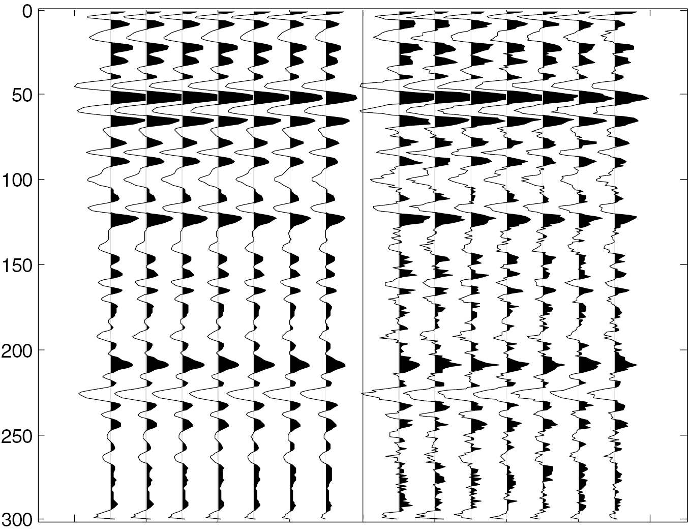
Standard image High-resolution imageSeismic data inevitably contains some noise, for this reason the noise that the SNR is 3 is added to synthetic seismic data for noise immunity test. Figure 5 shows the contrast of the data for inversion. The inversion results are shown in figures 6(a) and (b) corresponding to the LM and the new algorithm, respectively. P-wave velocity reflection coefficient, , shear wave velocity reflection coefficient, , and density reflection coefficient are demonstrated from left to right. Although overall inversion results in figure 6(a) keep a good consistency with the model value, the inversion result is better in figure 6(b). Inversion for density is unstable which is a bottleneck of three-parameter AVO inversion. However, a credible result can still be obtained. In summary, the new algorithm behaves better than LM for AVO inversion even through the conditions of the interface are quite different because of the high order approximation used in this study.


Figure 5. Synthetic seismic data and synthetic seismic data with noise (S/N = 3).
Download figure:
Standard image High-resolution image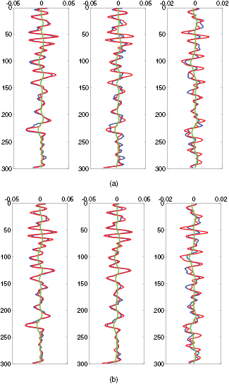
Figure 6. (a) Inversion value comparison by the LM algorithm. (b) Inversion value comparison by the new algorithm.
Download figure:
Standard image High-resolution imageIn some special circumstances seismic data with limited SNR is possible, as a result, more noise (S/N = 1) is considered in this work (figure 7). Figure 8 shows the inversion result when S/N is 1. It is feasible to achieve three-parameter inversion even though seismic data quality is unsatisfactory. Inversion values have a high correlation with the model values if an apposite initial model is given. Now please take a closer look at the initial models used in figures 6(b) and 8, where it is obviously the same for different noise. However, the LM algorithm is provided with a higher requirements as the noise increases. So the new algorithm has advantages and is effective and credible for solving nonlinear AVO inversion problems.

Figure 7. Synthetic seismic data and synthetic seismic data with niose (S/N = 1).
Download figure:
Standard image High-resolution image
Figure 8. Inversion result by new algorithm (S/N = 1).
Download figure:
Standard image High-resolution imageinfluences the inversion result especially for a reservoir where changes significantly. The red box in figures 9 and 10 locates a sand reservoir. Figure 9 shows the inversion results when , while figure 10 shows the inversion results when changes with time. It is noteworthy that the full Zoeppritz equation is utilized so that we do not need to consider in the forward modeling process, and the way of generating synthetic seismogram is more reasonable. As a result, a difference will happen because of different utilized during the inversion and a better inversion results are obtained when a changing is used.


Figure 9. Inversion results of when .


Download figure:
Standard image High-resolution image
Figure 10. Inversion results of when is changing with time.


Download figure:
Standard image High-resolution image5. Real data inversion
A model test lays the foundation for the actual data inversion. The seismic data is from China. Before pre-stack seismic inversion, seismic data requires amplitude preservation processing, including the proliferation compensation, calibration of source and detector combination effects, inverse Q filtering, surface consistent processing, pre-stack denoising, removal of multiple waves, and assuming multiples and anisotropy of interlayer processed are negligible (Zong 2012). Figure 11 shows three partial angle stacked seismic profiles with different center incidences. The vertical axis represents sampling point number, the horizontal axis is CDP and sample interval is 2 ms. The inversion results of are presented in figure 12 where the vertical axis represents time and the unit is in seconds. Then they are inverted to by trace integration (figure 13). The trace from inversion (blue) and the upscaled well-log (red) are plotted together in figure 14.


Figure 11. (a) Partial angle stacked seismic profile of small angle; (b) partial angle stacked seismic profile of mid angle; (c) partial angle stacked seismic profile of large angle.
Download figure:
Standard image High-resolution image
Figure 12. (a) Inversion value of ; (b) inversion value of ; (c) inversion value of .


Download figure:
Standard image High-resolution image
Figure 13. (a) Inversion value of ; (b) inversion value of ; (c) inversion value of .


Download figure:
Standard image High-resolution image
Figure 14. The trace from inversion and the upscaled well-log.
Download figure:
Standard image High-resolution imageInversion results are reasonable compared with the seismic data (figures 11 and 13). Due to the use of a variation of compressional and shear wave velocity ratio, the correlation of shear wave velocity profile and p-wave velocity profile decrease. The well position is the 150th CDP and the red part stands for low values. The inversion results for three parameters () are in good agreement with the well logs.

6. Conclusion
In this paper, inverse operator estimation in thr trust region algorithm is applied for AVO inversion. The inversion objective function takes advantage of thr higher-order Zoeppritz approximation equation and utilizes a changing compressional and shear wave velocity ratio. Model test results show that the new algorithm has higher stability and accuracy than the LM algorithm. Seismic inversion results also maintain good consistency with the actual data and log data. Overall, this AVO nonlinear inversion method has some practical value.
Acknowledgments
This work was jointly funded by National Natural Science Foundation of China Petroleum & Chemical Joint Fund Project (U1562215), China Postdoctoral Science Foundation (2014M550379), Shandong Province postdoctoral Innovation Fund (2014BSE28009) and Sinopec Geophysical Laboratory Fund (33550006-14-FW2099-0038).