Boundary fidelity and entanglement in the symmetry protected topological phase of the SSH model

This is the simplest case to handle. Taking the doubling of the unit cell due to the dimerization into account and performing a Fourier transform, the Hamiltonian (1.1) can be written as

$$\begin{equation} H=-2t\sum_{k}\left(\begin{array}{@{}c@{}}c_{1k}^\dagger \\\ms c_{2k}^\dagger\end{array}\right)^T \left(\begin{array}{@{}cc@{}}0 & \cos k+ {\rm i}\delta\sin k\\ \cos k - {\rm i}\delta\sin k & 0\end{array}\right) \left(\begin{array}{@{}c@{}}c_{1k} \\ c_{2k}\end{array}\right) \end{equation} \tag{ 2.1 }$$

where k = 2πn/N and n = 1, ···, N/2. This is straightforwardly diagonalized. The eigenvalues are

$$\begin{equation} \lambda^\pm_k=\pm 2t\sqrt{\cos^2 k+\delta^2\sin^2 k}=\pm \sqrt{2}t\sqrt{1+\delta^2+(1-\delta^2)\cos 2k} \end{equation} \tag{ 2.2 }$$

with a gap at the Fermi points k_F = ±π/2 given by Δ_E = 4t|δ|. The new operators in which the Hamiltonian is diagonal,

$$\begin{equation} H=-\sum_k \lambda^+_k \left(\alpha_k^\dagger\alpha_k -\beta_k^\dagger\beta_k\right)\, , \end{equation} \tag{ 2.3 }$$

are given by

$$\begin{equation} \alpha_k=\frac{1}{\sqrt{2}} (\mathcal{A} c_{k1} +c_{k2}),\quad \beta_k=\frac{1}{\sqrt{2}} (-\mathcal{A} c_{k1} +c_{k2}) \end{equation} \tag{ 2.4 }$$

with $\mathcal{A}=\lambda_k^+/[2t(\cos k+{\rm i}\delta\sin k)]$. The ground state of the Hamiltonian (2.3) at half-filling is obtained by filling up the valence band, $|\Psi_0\rangle = \prod_k \alpha_k^\dagger |0\rangle$.

While in the PBC case only two momentum modes are coupled so that we are left with the diagonalization of a 2 × 2 matrix, see equation (2.1), open boundary conditions instead lead to a coupling of all momentum modes so that a Fourier transform does not diagonalize the problem.

In real space, on the other hand, the Hamiltonian is a symmetric tridiagonal matrix with zero diagonal elements and superdiagonal and subdiagonal elements which alternate between 1 ± δ. The eigenvalues and -vectors are explicitly known if the number of lattice sites is odd [16]. The eigenvalues are

$$\begin{equation} \lambda_0 = 0, \quad \lambda^\pm_k = \pm \sqrt{2}t\sqrt{1+\delta^2+(1-\delta^2)\cos \theta_k} \end{equation} \tag{ 2.5 }$$

where

$$\begin{equation} \theta_k=\frac{2\pi k}{N+1} \end{equation} \tag{ 2.6 }$$

and k = 1, ···, (N − 1)/2. The spectrum thus contains a single zero energy mode, see figure 1(a). If we parametrize each eigenvector as

$$\begin{equation} |\psi_k\rangle=(x_1^k,x_2^k,\ldots,x_N^k)^{\rm T}\,, \end{equation} \tag{ 2.7 }$$

then the not-normalized elements of the eigenvector for the zero energy mode are

$$\begin{equation} \fl x^0_{2n-1}=\left(-\frac{1-\delta}{1+\delta}\right)^{n-1}, \; n=1,\cdots,\frac{N+1}{2};\quad x^0_{2n}=0,\; n=1,\cdots,\frac{N-1}{2}. \end{equation} \tag{ 2.8 }$$

For the other modes one finds

$$\begin{eqnarray} &&x^k_{2n-1} = \frac{1+\delta}{1-\delta}\sin\left(\frac{2\pi k(n-1)}{N+1}\right)+\sin\left(\frac{2\pi k n}{N+1}\right), \; n=1,\cdots, \frac{N+1}{2}\nonumber\\ &&x^k_{2n} = \frac{\lambda_k^\pm}{1-\delta}\sin\left(\frac{2\pi kn}{N+1}\right),\; n=1,\cdots,\frac{N-1}{2}. \end{eqnarray} \tag{ 2.9 }$$

Depending on the sign of the dimerization δ the edge mode is thus localized either at the right or the left end of the chain.

Zoom In Zoom Out Reset image size

For an even number of lattice sites we expect two edge states for δ > 0 and no edge states for δ < 0. The eigenenergies $\lambda_k^\pm$ can still be written as in equation (2.5), however, the parameters θ_k are no longer known analytically and instead have to be determined by numerically solving the implicit equation [16]

$$\begin{equation} (1-\delta)T(\theta_k,N/2)+(1+\delta)T(\theta_k,N/2-1)=0 \,, \end{equation} \tag{ 2.10 }$$

with

$$\begin{equation} T(\theta_k,n)=\frac{\sin[(n+1)\theta_k]}{\sin\theta_k}\,. \end{equation} \tag{ 2.11 }$$

The eigenvector corresponding to each of the N solutions θ_k of equation (2.10) is then given by

$$\begin{eqnarray} &&x_{2n-1}^k(\delta)=\frac{1+\delta}{1-\delta}T(\theta_k,n-2)+T(\theta_k,n-1)\nonumber\\ &&\hskip0.9pc x_{2n}^k(\delta)=\frac{\lambda^\pm_k}{1-\delta}T(\theta_k,n-1)\,, \end{eqnarray} \tag{ 2.12 }$$

where n takes values from 1, 2, ··· N/2.

While for δ < 0 all N states are extended, localized edge states are possible for δ > 0 corresponding to complex solutions of equation (2.10). More precisely, we find that the system has N − 2 real solutions and two complex solutions if δ > δ_c where

$$\begin{equation} \delta_c=\frac{1}{1+N}, \end{equation} \tag{ 2.13 }$$

while all solutions are real if δ < δ_c. Physically, this can be understood as follows: The extended states in a finite system are protected against a small dimerization by the finite size gap Δ_E of order 1/N. Only if the gap Δ_E ∼ |δ| induced by the dimerization overcomes the finite size gap can the spectrum change qualitatively. Alternatively, one can also think about this problem in terms of the localization length ξ_loc ∼ 1/δ of the edge state, see equation (2.8), which has to become smaller than the system size in order to allow for localized states. In the thermodynamic limit, N → ∞, we have δ_c → 0 so that the phase transition between the topological trivial and the SPT phase occurs, as expected, at δ = 0. The eigenspectrum for a finite system as a function of dimerization shown in figure 1(b) makes it clear that there is always a small gap between the two edge modes which will only go to zero for all δ > 0 in the thermodynamic limit.

In this case there is no boundary so that χ_B = 0. Furthermore, we expect χ(δ) = χ (−δ) for N even because changing the sign of δ is in this case equivalent to a simple relabelling of the lattice sites.

Using the results of section 2.1, the analytic calculation of the fidelity at half-filling is straightforward

$$\begin{eqnarray} \fl|\langle \Psi(\delta)|\Psi(\delta+\epsilon)\rangle| &=& \prod_{k,k^\prime} |\langle 0 | \alpha_k\tilde\alpha_{k^\prime}^\dagger |0\rangle | \\ \fl&=& \frac{1}{2}\prod_{k,k^\prime} |\langle 0 | (\mathcal{A}c_{1k}+c_{2k})(\tilde{\mathcal{A}}^*c^\dagger_{1k^\prime}+c^\dagger_{2k^\prime}) |0\rangle | \nonumber\\ \fl&=& \prod_k \frac{|\mathcal{A}\tilde{\mathcal{A}}^*+1|}{2} \nonumber \end{eqnarray} \tag{ 3.6 }$$

where $\tilde\alpha_k$ and $\tilde{\mathcal{A}}$ are obtained by replacing δ → δ + . For the fidelity density this leads to

$$\begin{equation} f=-\frac{1}{N}\sum_k\ln\frac{|\mathcal{A}\tilde{\mathcal{A}}^*+1|}{2} \stackrel{N\to\infty}{\to} -\frac{1}{\pi}\int_0^{\pi/2}\ln\frac{|\mathcal{A}\tilde{\mathcal{A}}^*+1|}{2} {\rm d}k \, . \end{equation} \tag{ 3.7 }$$

The bulk fidelity susceptibility can now be calculated in closed form

$$\begin{equation} \chi_0=\frac{1}{32\pi}\int_0^{\pi/2}{\rm d}k\frac{\sin^2 2k}{(\cos^2 k+\delta^2\sin^2 k)^2} = \frac{1}{32|\delta|(1+|\delta|)^2}\, . \end{equation} \tag{ 3.8 }$$

The finite size corrections in the gapped phase are exponentially small, χ(N) − χ₀ ∼ N exp(−N/ξ) for N ≫ 1, where ξ is the correlation length, see equation (4.14). At the critical point δ = 0 the fidelity susceptibility thus diverges as χ₀ ∼ 1/|δ|. This is consistent with the general scaling theory at a critical point δ_c which predicts χ₀ ∼ |δ − δ_c|^dν−2 where d is the spatial dimension and ν the critical exponent related to the divergence of the correlation length at the critical point. In the case considered here we have δ_c = 0, d = 1 and ν = 1.

In the open chain case, we expect a 1/N boundary contribution χ_B (surface term) to the fidelity susceptibility. According to the bulk-boundary correspondence, a symmetry protected topological phase as indicated by a bulk invariant Zak-Berry phase is related to the presence of edge modes. We thus expect that χ_B is a measure which can distinguish between a topologically trivial and a non-trivial phase.

We start by considering the case of an odd number of sites N where the single particle eigenstates are known exactly, see section 2.2. Note that in this case a single edge mode is present both for δ < 0 and for δ > 0. In order to obtain both the bulk and the boundary contribution, we use equations (3.3)–(3.5) with the exact single particle eigenstates given by equations (2.8) and (2.9). We are interested in the half-filled case, however, for N odd we can only put either (N − 1)/2 or (N + 1)/2 particles into the system. This means that the zero energy edge mode is either empty or occupied. Because the Hamiltonian is particle-hole symmetric, the fidelity is, however, exactly the same in both cases.

In figure 2 we show exemplarily the scaling of the fidelity susceptibility for different dimerizations, demonstrating that the leading correction to the bulk susceptibility is indeed of order 1/N. The bulk and boundary susceptibilities extracted from the scaling are shown in figure 3. Note that both are symmetric in δ as they should be because δ → −δ is—up to a relabelling of the lattice sites—a symmetry of the Hamiltonian (1.1) if N is odd. The bulk contribution χ₀ is independent of the boundary conditions and agrees with the analytical solution (3.8) obtained using periodic boundary conditions. For the boundary contribution χ_B we numerically find a behaviour close to the critical point which is consistent with χ_B ∼ 1/|δ|^η with η ≈ 2. Note, however, that we have two different edges for the N odd case which can give boundary contributions which scale differently. The analysis of χ_B is therefore easier in the N even case considered next where either both edges have a localized state or both are trivial.

Zoom In Zoom Out Reset image size

Zoom In Zoom Out Reset image size

In the N even case we can again calculate the overlap matrix (3.4) from the single particle eigenstates, equation (2.12). However, this time the parameters θ_k have to be determined by the implicit equation (2.10). Especially for the bound states where θ_k becomes imaginary this requires a high accuracy making the calculations numerically challenging for large system sizes.

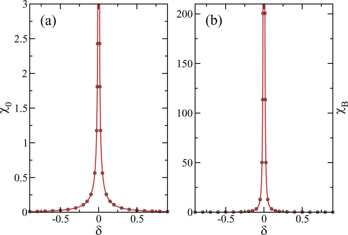
The boundary susceptibility obtained in this case is shown in figure 4. Note that χ_B in the topological trivial phase (δ < 0) is qualitatively different from χ_B in the SPT phase (δ > 0). In particular, the sign is different. The data in figure 4(b), furthermore, indicate that also the exponents of, what seems to be a power-law divergence at the critical point, are different by about 5%. The presence or absence of edge states is thus clearly visible in χ_B.

Zoom In Zoom Out Reset image size

For large chain lengths N the edges should become independent so that χ_B is simply the sum of the contributions from each of the two edges. In particular, this implies that

$$\begin{equation} \left[\chi_B^{N\;{\rm even}\to\infty}(\delta) + \chi_B^{N\;{\rm even}\to\infty}(-\delta)\right]/2 = \chi_B^{N\; {\rm odd}\to\infty}(\pm\delta). \end{equation} \tag{ 3.9 }$$

This behaviour is confirmed by the fits shown in figure 4(b). The data for the N odd case are thus better fitted by the sum of two power laws with different exponents rather than by the single power law used in figure 3.

Finally, we can also study the finite size scaling of the fidelity susceptibility right at the critical point, see figure 5. While both data sets for N even and N odd show a scaling χ ∼ N consistent with the general scaling prediction χ ∼ N^2/dν−1 [20], the prefactors are different.

Zoom In Zoom Out Reset image size

To summarize, we have established that the boundary susceptibility χ_B behaves qualitatively different in the SPT (δ > 0) than in the topologically trivial phase (δ < 0). In particular, χ_B(δ < 0) < 0 and χ_B(δ > 0) > 0.

In the following, we want to study the entanglement entropy of the SSH model (1.1). We will consider two cases: First, a block in an infinite chain. Here we can simply use PBC which makes it possible to perform the thermodynamic limit exactly. This case will provide a numerical check of the formula (4.6). Second, we will consider the case of a block at the end of a semi-infinite chain. Here we can use either odd chain lengths where the eigenstates are known explicitly, or even chain lengths. The odd chain length has an edge state which is either filled or empty, which are equivalent by particle-hole symmetry. In contrast at half-filling a finite open system with an even number of sites in the SPT phase has two edge states, only one of which is occupied at half filling. However, the boundary states at the edges in the thermodynamic limit are a superposition of states localized at the left and the right edge. Thus we can also consider a semi-infinite chain with a partially occupied edge state. Since the correlation length ξ ∼ |δ|⁻¹ is finite for δ ≠ 0 it suffices to consider chain lengths N ≫ ξ in order to be effectively in the thermodynamic limit. We are particularly interested in the difference in entanglement entropies with and without a localized state being present at the boundary of the chain.

For a free fermion model there is a general setup to obtain the eigenvalues of the reduced density matrix ρ_A [35, 36]. The main observation is that ρ_A can be represented as the exponential of a free-fermion operator $\mathcal{H}_A$—the so-called entanglement Hamiltonian—with

$$\begin{equation} \rho_A = \frac{1}{\mathcal{Z}}\exp(-\mathcal{H}_A)=\frac{1}{\mathcal{Z}}\exp\left(-\sum_{k=1}^\ell\epsilon_k a_k^\dagger a_k\right) \end{equation} \tag{ 4.7 }$$

and $\mathcal{Z}={\rm Tr}\exp(-\mathcal{H}_A)$. On the other hand, all properties of a free-fermion system can be obtained from the matrix C of two-point correlation functions because all higher correlation functions can be expressed through the two-point functions by using Wick's theorem. The matrix elements of C for all two-point functions within the considered block A are, in particular, determined by the reduced density matrix ρ_A, i.e. matrix elements are given by

$$\begin{equation} C_{ij}={\rm Tr}(\rho_A c_i^\dagger c_j) \,. \end{equation} \tag{ 4.8 }$$

The eigenvalues ζ_k of the correlation matrix can then be related to the eigenvalues _k of the entanglement Hamiltonian in equation (4.7) and one finds

$$\begin{equation} \zeta_k = ({\rm e}^{\epsilon_k}+1)^{-1}. \end{equation} \tag{ 4.9 }$$

According to equation (4.7) the 2^ℓ-many eigenvalues z_p of ρ_A itself are now obtained by considering all possible fillings of the ℓ-many levels _k

$$\begin{equation} z_p=\frac{1}{\mathcal{Z}}\prod_k\exp\left(-\epsilon_k n^{(p)}_k\right) \end{equation} \tag{ 4.10 }$$

where $n^{(p)}_k\in \{0,1\}$ are fixed single-level occupation numbers, and $\mathcal{Z}=\sum_p z_p$. The entanglement entropy is then given by

$$\begin{equation} S_{\rm ent}=-\sum_p z_p \ln z_p. \end{equation} \tag{ 4.11 }$$

Using the results from section (2.1) for a chain with PBC at half-filling, the two-point correlation function can be easily calculated and the thermodynamic limit performed exactly. For even distances one finds C_ij = δ_ij/2, i.e. only the onsite correlation function (occupation number) is nonzero. For odd distances the result is

$$\begin{equation} \fl \langle c^\dagger_{2n}c_{2m+1}\rangle =\frac{1}{2\pi}\int_{-\pi/2}^{\pi/2} {\rm d}k \frac{\cos k\cos k(2m+1-2n)+\delta\sin k\sin k(2m+1-2n)}{\sqrt{\cos^2k +\delta^2\sin^2 k}} \end{equation} \tag{ 4.12 }$$

and the correlation function $\langle c^\dagger_{2n+1}c_{2m}\rangle$ is obtained by replacing δ → −δ. For the non-dimerized case, this reduces to the well-known result

$$\begin{equation} \langle c^\dagger_{n}c_{m}\rangle =\frac{1}{\pi}\frac{\sin\left[\frac{\pi}{2}(m-n)\right]}{m-n} \,. \end{equation} \tag{ 4.13 }$$

By methods of steepest descent we can also obtain the asymptotic behaviour of the correlation function (4.12) at large distances. In particular, we find that the dominant correlation length is given by

$$\begin{equation} \xi^{-1}\equiv \xi_1^{-1}=\frac{1}{2}\left|\ln\frac{1+\delta}{1-\delta}\right| \,. \end{equation} \tag{ 4.14 }$$

There should now be three different regimes depending on the ratio of block size ℓ and largest correlation length ξ ≡ ξ₁: (1) For ξ ≫ ℓ ≫ 1 the entanglement entropy will essentially follow the scaling law for a critical system, equation (4.2), as obtained by CFT. Exemplarily, we present in figure 6 results for S_ent for small dimerizations and odd block lengths ℓ. Indeed, we see that the smaller the dimerization is the longer equation (4.2) approximately holds as a function of block size. (2) For ξ ≪ ℓ, on the other hand, the entanglement entropy will settle to a constant value $S_{\rm ent}=\frac{c}{3}\ln(\xi/a)+U$ where both constants a and U are non-universal. This behaviour is shown exemplarily in figure 7(a). In figure 7(b) we show, furthermore, that the saturation value depends on whether two weak bonds (ℓ even), a weak and a strong bond (ℓ odd), or two strong bonds (ℓ even) are cut. We have chosen the block for ℓ even in such a way that δ < 0 corresponds to cutting two weak and δ > 0 to cutting two strong bonds. For block sizes ℓ≫ξ each non-trivial edge—caused by the cutting of a strong bond—gives an independent contribution S_edge to the entanglement entropy. More precisely, we can define the edge contribution as

$$\begin{equation} S_{\rm edge}=\lim_{\ell\to\infty}|S_{\rm ent}(\ell,\; \ell\;{\rm odd})-S_{\rm ent}(\ell+1,\; \ell+1\; {\rm even})|, \end{equation} \tag{ 4.15 }$$

which is shown as a function of dimerization in figure 8. In particular, in the limit |δ| → 1 the entanglement entropy will be dominated entirely by the edge contribution so that $S_{\rm ent}^{\delta\to 1}(\ell\; {\rm even})=2 S_{\rm edge}^{\delta\to 1}$, $S_{\rm ent}^{\delta\to 1}(\ell\; {\rm odd})=S_{\rm edge}^{\delta\to 1}$ and $S_{\rm ent}^{\delta\to -1}(\ell\; {\rm even})\equiv0$ with $S_{\rm edge}^{\delta\to 1}=\ln 2$. The insets of figure 8 are consistent with a power law behaviour of S_edge for small δ and for δ → 1.

Zoom In Zoom Out Reset image size

Zoom In Zoom Out Reset image size

Zoom In Zoom Out Reset image size

(3) Finally, there is also the regime ξ≲ℓ where the formula (4.6) should hold which gives the leading correction to the constant value obtained in the limit ξ≪ℓ. In the case of the dimerized model considered here, the leading correlation length ξ will show up twice: once with wave vector k = π/2 and once with wave vector k = −π/2 [37, 38]. Therefore, to leading order, we expect the entanglement entropy to scale as

$$\begin{equation} S_{\rm ent}=S_{\rm ent}(\ell\to\infty)-\frac{1}{4}K_0(2\ell/\xi) \end{equation} \tag{ 4.16 }$$

with ξ as given in equation (4.14). Fixing S_ent(ℓ → ∞) by the numerical data for large block sizes, there is thus no free fitting parameter. The comparison in figure 9 with data for |δ| = 0.02, in which case ξ ≈ 25, confirms this scaling prediction. For large arguments, the Bessel function asymptotically scales as $K_0(x)\sim\sqrt{\frac{\pi}{2x}}\exp(-x)$. The inset of figure 9 demonstrates that this is indeed the correct scaling of the entanglement entropy for large block sizes. The data for the three different cuts, in particular, collapse onto a single line after subtracting the constant part S_ent(ℓ → ∞).

Zoom In Zoom Out Reset image size

To calculate the entanglement entropy for a block which includes the end of a semi-infinite chain, we can use the analytic results for the single-particle eigenstates of a chain with OBC and N odd given in section 2.2 and the numerical results for N even from section 2.3. In both cases, the matrix elements of the correlation matrix C_ij, see equation (4.8), can be expressed as

$$\begin{equation} C_{ij}=\sum_{k\;\, {\rm occupied}} (\Psi^k_i)^* \Psi^k_j \end{equation} \tag{ 4.17 }$$

with the sum running over all occupied single-particle states. Diagonalizing the correlation matrix then gives access to the single-particle eigenenergies _k of the entanglement Hamiltonian using the relation (4.9).

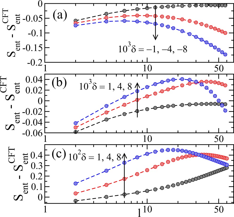
Results for small dimerizations are shown in figure 10. While the entanglement entropy for δ < 0, where a strong bond terminates the semi-infinite chain, behaves qualitatively similar to the case of a block in an infinite chain (see figure 6) we find a much more complicated scaling for δ > 0 and N odd. In this case a localized boundary state is present leading to a competition between an increase of the boundary contribution to S_ent with increasing δ and a decrease of the bulk contribution due to the decreasing correlation length ξ ∼ 1/δ. As a result, the curves for different dimerizations cross, see figure 10(b).

Zoom In Zoom Out Reset image size

The final possibility is to consider the semi-infinite chain with a localized edge state which is not fully occupied, as realized in a chain N even at half-filling, see figure 10(c). As for the fully occupied edge state there is a competition between the increasing boundary entropy and decreasing bulk entropy with δ. However, due to the higher degeneracy associated with the partially occupied edge state, see also the entanglement spectra in the following section, the curves for the same dimerizations will cross at a much larger sub-block size, than for a fully occupied edge state. Therefore we show in figure 10(c) data for dimerizations which are an order of magnitude larger than in the other two cases shown in figures 10(a) and (b).

For large block size ℓ and finite dimerization we again expect that S_ent saturates. Let us first concentrate on the case δ < 0 shown in figure 11. In this case S_ent is monotonically increasing. We can thus try to fit the data for large block sizes by

$$\begin{equation} S_{\rm ent} = S_{\rm ent}(\ell\to\infty)-\frac{1}{8} K_0(2\ell/\tilde\xi) \end{equation} \tag{ 4.18 }$$

similar to the quantum field theory result (4.6) but with $\tilde\xi$ as a free parameter. Doing so we obtain very good fits with parameters as given in table 1. The correlation length $\tilde\xi$ obtained from the fits seems to be about a factor $\sqrt{2}$ smaller than the bulk correlation length ξ given in equation (4.14). Note, however, that the heuristic fitting formula (4.18) is too naive to be able to fully capture the behaviour of S_ent. A two-point correlation function near a boundary does not only depend on the distance between the two operators but also on the distance of the operators from the boundary so that a third length scale has to appear.

Zoom In Zoom Out Reset image size

Table 1. Parameters in equation (4.18) used to fit the data for large block sizes shown in figure 11.

δ	Sent(ℓ → ∞)	$\tilde\xi$	ξ	$\xi/\tilde\xi$
−0.02	0.838	34.80	49.99	1.44
−0.04	0.696	17.59	24.99	1.42
−0.06	0.605	11.89	16.65	1.40

Let us now return to the case δ > 0 with the fully occupied boundary state where figure 10(b) already indicates that the scaling behaviour of the entanglement entropy with block size is completely changed. Figure 12 shows that the competition between boundary and bulk contributions leads to a maximum in S_ent which becomes sharper and whose position shifts to smaller block sizes with increasing dimerization. Consequently, the constant value S_ent(ℓ → ∞) is now approached from above. Clearly a scaling as in (4.18) is no longer valid.

Zoom In Zoom Out Reset image size

To verify that the additional entanglement entropy is indeed caused by the boundary state we can define

$$\begin{equation} S_{\rm bound}(\ell) = S^{\delta>0}_{\rm ent}(\ell,\, \ell\, {\rm odd}) - S^{\delta<0}_{\rm ent}(\ell+1,\, \ell+1 \, {\rm even})\;. \end{equation} \tag{ 4.19 }$$

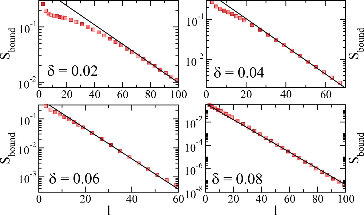
For both entropies in equation (4.19) a weak bond is cut so that for large block sizes ℓ any remaining difference is directly related to the localized boundary state present for δ > 0. Figure 13 shows that S_bound(ℓ) is exponentially decaying with block size. According to equation (2.8) a non-trivial boundary leads to an exponentially localized zero energy state with a localization length

$$\begin{equation} \xi^{-1}_{\rm loc}=\ln\left(\frac{1+\delta}{1-\delta}\right). \end{equation} \tag{ 4.20 }$$

The exponential fits in figure 13 using this correlation length are indeed in excellent agreement with the data for S_bound(ℓ) confirming that the boundary state leads to additional entanglement which is exponentially localized at the boundary.

Zoom In Zoom Out Reset image size

For δ > 0, N even and half-filling the boundary state is only half-filled. As shown in figure 14 this qualitatively changes the behaviour of S_ent as compared to the case where the edge state is completely filled. In particular, there is no longer a maximum yet the scaling with block size is also not described by a modified Bessel function as was the case for δ < 0. Instead, the scaling seems purely exponential

$$\begin{equation} S_{\rm ent}(\ell)=S_{\rm ent}(\ell \rightarrow\infty)-a\exp(-2\ell/\xi) \end{equation} \tag{ 4.21 }$$

with ξ being the leading correlation length, see equation (4.14) and a a fitting parameter. The boundary contribution of the partially filled edge state can again be calculated from equation (4.19) and is exponentially decaying with block size similar to the case of the completely filled edge state, see figure 15. To summarize, we have shown that the presence of localized boundary states in a massive phase completely changes the scaling of S_ent(ℓ) with block size ℓ for a block at the end of a semi-infinite chain. The boundary state leads, in particular, to additional entanglement which is exponentially loacalized. Further insight into the different entanglement properties of a block with or without a localized boundary state can be gained by directly investigating the entanglement spectrum.

Zoom In Zoom Out Reset image size

Zoom In Zoom Out Reset image size

As for the entanglement entropy we can use the analytical result for the elements of the correlation matrix in the thermodynamic limit to determine the spectrum of the reduced density matrix. In figure 16 the logarithm of the eigenvalues z_p of the reduced density matrix, see equation (4.10), for the three different cuts possible are shown. The pictograms in the figure show whether the block size is even or odd (but not the actual block size!) and if strong (double lines) or weak (single dashed lines) bonds are cut. While the structure is complicated for finite block sizes ℓ, the distribution of eigenvalues becomes very simple in the limit ℓ → ∞. In this case, the single particle energies _k of the entanglement Hamiltonian (4.7) become equally spaced and the level spacing can be obtained analytically using corner transfer methods [24, 39]. One finds

$$\begin{equation} \epsilon=\pi I(x^\prime)/I(x) \quad {\rm with}\ x=(1-\delta)/(1+\delta), \end{equation} \tag{ 5.1 }$$

$x^\prime=\sqrt{1-x^2}$ and I(x) being the elliptic integral of the first kind. This is the correct level spacing for odd block size as well as for even block size if two weak bonds are cut. Cutting two strong bonds, on the other hand, leads to a level spacing 2, see figure 16.

Zoom In Zoom Out Reset image size

The eigenvalues z_p of the reduced density matrix in the thermodynamic limit can then be obtained by filling up the single particle levels. The dominant eigenvalue of ρ_A is obtained by filling up the 'Fermi sea' of negative eigenvalues _k. In the case shown in figure 16(b)—where the block size is even and two weak bonds are cut—this leads to a unique dominant eigenvalue. In the case where either one (figure 16(a)) or two (figure 16(c)) strong bonds are cut the lowest eigenvalue is, however, degenerate. This can be understood as follows: Cutting a strong bond leads to an edge spin. For the case ℓ odd where one strong bond is cut this leads to an eigenenergy _(ℓ+1)/2 ≡ 0. This level can now either be empty or filled leading to a two-fold degeneracy of the leading eigenvalue. For the case ℓ even where two strong bonds are cut, eigenvalues _ℓ/2 = −_ℓ/2+1 appear which approach zero in the thermodynamic limit. Consequently, the dominant eigenvalue of ρ_A becomes four-fold degenerate. Thus the low-energy entanglement spectrum allows to directly identify the number of 'edge states' caused by cutting a strong bond.

Equation (5.1) only gives the level spacing. In order to obtain the allowed values for the eigenvalues z_p of ρ_A one has to use, in addition, the normalization condition

$$\begin{equation} 1= {\rm Tr}\rho_A=\sum_p z_p =\sum_{k=0}^\infty {\rm d}_k {\rm e}^{-\epsilon_0-k\epsilon} \Rightarrow \epsilon_0=\ln\left(\sum_{k=0}^\infty {\rm d}_k {\rm e}^{-k\epsilon}\right). \end{equation} \tag{ 5.2 }$$

Here d_k is the number of degenerate eigenvalues {z_p} for which z_p = exp(−₀ − k) with k fixed. The levels ₀+k or ₀ + 2k, respectively, with k = 0, 1, 2, 3, ··· are shown as dashed lines in figure 16.

While the case of a block in an infinite chain is well understood, the interesting case of the entanglement spectrum for a block at the end of a dimerized semi-infinite chain with or without a localized boundary state has not been considered so far. We have already shown that a localized boundary state causes additional entanglement which is also localized at the boundary, see figure 13. Here we want to further investigate this case by directly looking at the entanglement spectrum.

For N odd, we can distinguish four cases now: δ < 0 (topological trivial case) or δ > 0 (SPT case) with ℓ either even or odd. In addition, we have to consider the two cases ℓ even or odd with N even and δ > 0, where the edge state is only partially filled, separately. We start with the topological trivial case δ < 0. Data for even and odd block sizes with δ = −0.1 are shown in figure 17. For even block sizes, see figure 17(a), the leading eigenvalue is unique and the separation of the single-particle levels is given by equation (5.1) as in the case of an even block in an infinite chain where two weak bonds are cut, see figure 16(b). However, the degeneracy structure of the higher levels is different which explains the differences in the entanglement entropy discussed in the previous subsection. For the case of an odd block size, shown in figure 17(b), the degeneracy structure of the spectrum is the same as for a block of odd length in an infinite chain, see figure 16(a), however, the level spacing in the semi-infinite chain is 2 instead of for the infinite chain. Note that the finite size corrections for a block at the end of a semi-infinite chain in the topological trivial case are of similar magnitude as for the infinite chain, i.e. for the lowest single-particle levels the data for the smaller block sizes ℓ = 19, 20 and the larger ones, ℓ = 69, 70, hardly deviate from each other.

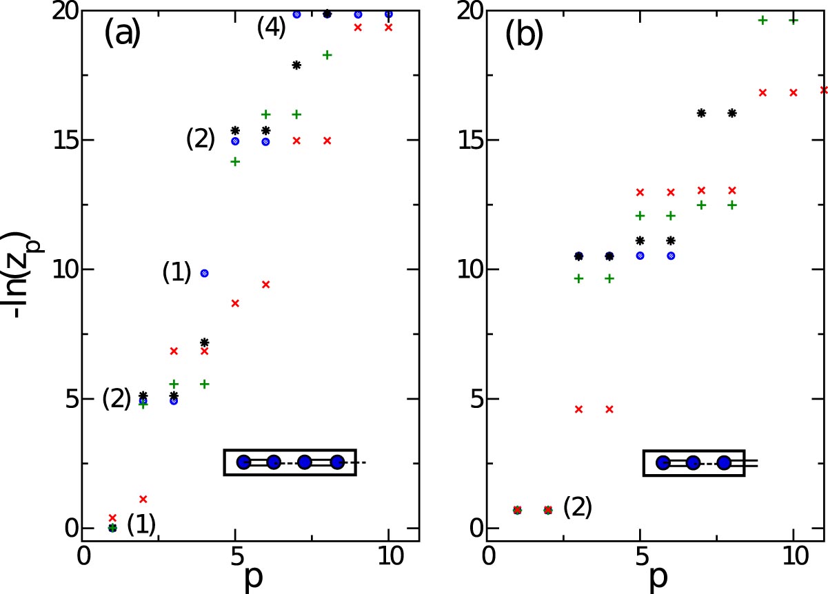
Zoom In Zoom Out Reset image size

This is completely different in the SPT phase—the case δ = 0.1 with N odd is shown as example in figure 18—where finite size corrections are much larger. In the limit ℓ → ∞, on the other hand, both the level spacing and the degeneracies agree between the cases δ < 0, ℓ even (figure 17(a)) and δ > 0, ℓ odd (figure 18(a)) as well as δ < 0, ℓ odd (figure 17(b)) and δ > 0, ℓ even (figure 18(b)). This means that the localized boundary state present for δ > 0 does not play any role in the limit ℓ → ∞ and that the spectra in the trivial and the SPT phase become identical in this limit.

Zoom In Zoom Out Reset image size

The dramatic change in the entanglement spectra for small block sizes if a localized state is present—which leads to the non-monotonic behaviour of the entanglement entropy shown in figure 12—can be understood as follows: The non-trivial edge leads to an exponentially localized zero energy state, equation (2.8), with a localization length as given in equation (4.20).

For the case δ = 0.1 considered here the localization length is ξ_loc ≈ 1/2δ = 5 lattice sites. The low-energy part of the entanglement spectrum will thus become similar to the one without the localized state if ℓ ≫ ξ_loc while it will be substantially modified for ℓ ≲ ξ_loc. The modification of the entanglement spectrum and the entanglement entropy is thus an effect of finite block size which is directly tied to the appearance of localized states in the SPT phase.

The final possibility is to consider the case N even, δ > 0 where the boundary state is only partially filled, see figure 19. In this case the degeneracy of the levels is doubled compared to the case with a fully occupied boundary state, shown in figure 18. Furthermore, corrections to the ℓ → ∞ limit for finite blocks are smaller, explaining the different behaviour seen in the entanglement entropy.

Zoom In Zoom Out Reset image size

To summarize, we have shown that the presence of a localized boundary state significantly alters the entanglement spectra for small block sizes. In the limit ℓ → ∞, on the other hand, a free fermion spectrum with an equidistant level spacing is recovered. While creating virtual edges by considering a block in an infinite chain gives the same degeneracy of the lowest level than a physical edge for a corresponding block at the end of a semi-infinite chain, the degeneracies of higher levels as well as the level spacing are, in general, different. This explains the different scaling properties of S_ent(ℓ) for a block at the end as compared to a block in the middle.

In figure 20 we show the fidelity susceptibility at different interaction strengths U for δ = 0.5 (topological phase for U = 0) and δ = −0.5 (trivial phase for U = 0). For U = 0.5 and U = 2.5 the fidelity susceptibility behaves qualitatively similar to the non-interacting case with the bulk susceptibility χ₀ being reduced with increasing interaction strength. Furthermore, we still find χ_B(δ < 0) < 0 and χ_B(δ > 0)>0 with χ_B given by the slope of the curves in figure 20 for 1/N small. This is an indication that the two cases remain topologically distinct even for intermediate interaction strengths. For U = 5, however, a drastic change is observed. In this case χ_B is negative both for δ < 0 and for δ > 0. Apparently the boundaries now behave qualitatively similar suggesting that a phase transition has occurred and edge states no longer exist. We will provide further evidence that this is indeed the case in the following. χ_B can thus be used as a measure to distinguish between phases with and without edge states also in interacting systems.

Zoom In Zoom Out Reset image size

We now turn to the entanglement spectra in the interacting case. We concentrate on large dimerizations (as an example, data for |δ| = 0.5 are shown throughout this section) where the correlation length is small so that effects caused by the finite chain length can be neglected for the low-energy part of the spectrum. As in the non-interacting case, we start by choosing a block from the middle of the chain, cutting (a) a weak and a strong bond, (b) two weak bonds and (c) two strong bonds, see figure 21. For weak and intermediate interaction strengths, U = 0.5 and U = 2 respectively, the degeneracy of the lowest level is not altered while for U = 10 a twofold degeneracy starts to emerge in all three cases. This can be understood as follows: For U/t → ∞ the ground state of the chain will become a superposition of the two degenerate product states, $|\Psi\rangle = (|1010\cdots 10\rangle + |0101\cdots 01\rangle)/\sqrt{2}$, i.e. the system is driven into a symmetrized CDW state ('cat state'). The reduced density matrix for any cut has then two eigenvalues 1/2 while all other eigenvalues are zero. The corrections for non-zero t/U ≪ 1 can be calculated perturbatively similar to the case of the XXZ chain considered in [24, 42]. The entanglement spectrum will then become equidistant again—though not all levels are necessarily occupied—with degeneracies which depend on the way the block is chosen and which are different from the non-interacting case. We thus expect an evolution with increasing U from an equidistant spectrum at U = 0 through some intermediate regime into a different equidistant spectrum at U/t ≫ 1. Such an evolution is indeed observed, see in particular figure 21(b), where already at U = 10 the spectrum becomes again almost equidistant.

Zoom In Zoom Out Reset image size

Next we plot the entanglement spectrum for a block at the end of a chain, a measure which is sensitive to the presence of localized edge states. First, we consider the evolution of the spectrum in what is the topological trivial phase for U = 0, see figure 22, cutting (a) a weak bond and (b) a strong bond. Again we find that the degeneracy of the lowest level is stable up to intermediate interactions, U = 2, while a new level structure with a twofold degenerate ground state emerges in both cases for U = 10.

Zoom In Zoom Out Reset image size

For a block at the end of a chain in the SPT phase, shown in figure 23, the picture is qualitatively similar. The boundary susceptibility and entanglement spectra for δ < 0 and δ > 0 thus remain distinct from each other even if nearest-neighbour interactions of intermediate strength are added. In particular, we still find numerically a twofold (fourfold) degeneracy of the lowest level for a block with ℓ odd (ℓ even) at the end of a chain in the SPT phase, see figure 23. For U = 0 this is directly related to an edge state which is shared between the two boundaries and which is thus, for an infinite separation of the boundaries, only partially filled.

Zoom In Zoom Out Reset image size

The LCRG algorithm is a variant of the density-matrix renormalization group [41, 43]. Originally proposed to study the real time evolution after a quantum quench, it is also possible to consider an imaginary time evolution starting from an initial product state. In this case the initial state is projected onto the ground state of the Hamiltonian used in the time evolution and ground state properties of infinite chains can be studied. Here we will use this algorithm to investigate the entanglement spectrum and entropy of an essentially infinite block within the infinite chain as a function of dimerization δ and interaction U. We choose our block in such a way that two strong bonds are cut so that the largest eigenvalue of the reduced density matrix for U = 0 will be fourfold degenerate. In figure 21 we have seen that this fourfold degeneracy changes into a twofold degeneracy at large interaction strengths. In order to find the point where this change occurs, we order the eigenvalues of the reduced density matrix by magnitude and plot LCRG results for 3z₁ − z₂ − z₃ − z₄ in figure 24(a). This quantity is zero as long as the largest eigenvalue is fourfold degenerate while it should become non-zero in the CDW phase. Indeed, a very sharp transition is observed numerically with U_c ≈ 4 at δ = 0.1 and U_c ≈ 8 for δ → 1. Since the symmetries which protect the SPT phase are not violated by the interaction, the excitation gap should close at the phase transition. To confirm a closing of the energy gap at the transition, we show the numerically calculated entanglement entropy as a function of U for various dimerizations δ in figure 24(b). The entanglement entropy evolves in all cases shown from S_ent ≈ 2ln 2 at U = 0 to S_ent = ln 2 for U → ∞. At U values consistent with those where we find an abrupt change of the degeneracy of the largest eigenvalue, see figure 24(a), the entanglement entropy has a sharp maximum. Here a comment about the numerical calculations is in order: We time evolve the initial product state up to imaginary times τ = 50. For all U values apart from the small region where S_ent is peaked the projection converges and the values shown in figure 24(b) are the finite fully converged entropies of the gapped ground states. At the phase transition, however, we find S_ent ∼ lnτ consistent with a diverging entanglement entropy for τ → ∞ as expected for a gapless state. In this case the projection is not fully converged and the values for S_ent shown are simply the values obtained at our maximal simulation time τ = 50.

Zoom In Zoom Out Reset image size