


Abstract.
Explosive synchronization (ES) on heterogenous networks is a hot topic in the study of complex networks in recent years. In this paper, we introduce an analytical framework to study the ES of Kuramoto oscillators on a star configuration, which is a simple and special heterogenous network. By using the Ott–Antonsen ansatz, we obtain a reduced set of low-dimensional equations for the macroscopic evolution of the system considered. Analysis of this reduced system theoretically confirms that the phase transition of the order parameter is indeed discontinuous. We also extend the problem studied to a general case with frequencies perturbation. The results show the phase transition is still discontinuous when the perturbations are small, and it degenerates to a continuous transition while the perturbation width exceeds a critical value. Numerical simulations show good agreement with the theoretical predictions. Our work provides an insightful perspective to understand the ES phenomena in large ensembles of coupled units.
Export citation and abstract BibTeX RIS
1. Introduction
Synchronization phenomena, which describe the emergence of collected behavior of large ensembles of coupled units, are always the focus of the intense research in synthetic and natural systems [1–3]. In 1998, Watts and Strognatz showed that the synchronization dynamics were strongly influenced by the structure of the interaction between the units in their seminal work [4], which was the seed of the modern theory of complex networks [5–7]. Since then, the synchronization processes with non trivial interaction patterns have been widely studied [8]. The main interest of these studies was the phase transitions from the incoherent states to the synchronized states, and it has been proven that these phase transitions are usually second-order [8].
In 2011, Gómez-Gardeñes et al [9] found that an explosive synchronization (ES) transition occurs on a scale-free (SF) network [6] for the Kuramoto model [10, 11] when the frequencies of oscillators positively correlate to the degrees of nodes. ES soon attracted many researchers' interest and become a hot topic in the study of dynamics on complex networks. Subsequent papers have further explored the influences of degree-frequency correlations [12, 13] and network structures [14, 15] on ES. ES has also been extended to some other models, such as Rössler units [16] and the weighted Kuramoto model [17]. These studies have greatly improved our understanding about many aspects of ES. However, as far as we know, the intrinsic mathematical mechanism of the emergence of ES on heterogenous networks has not been well clarified yet. To uncover this puzzle, an analytical framework that can deal with the high dimensional equations of the motion of the oscillators system is needed.
Ott and Antonsen introduced an ansatz to study the low dimensional behavior of global coupled Kuramoto oscillators in [18]. Using this anstaz, they derived a finite set of nonlinear ordinary differential equations for the macroscopic evolution of the system, and obtained a closed form solution for the Kuramoto oscillators with a Lorentzian frequency distribution. This anstaz has proven to be very efficient to solve the Kuramoto model and its variants, such as the Kuramoto model with phase lag [19], time delay [20] and bimodal frequency distribution [21].
In this paper, we use the Ott–Antonsen ansatz to study the time evolution of ES of Kuramoto oscillators. For the sake of mathematical treatment, we reduce the problem studied to the analysis of the star configuration, a special structure that grasps the main property of SF networks, namely, the role of hubs. The main work in this paper consists of two parts. Part one (section 2) discusses the time evolution of the Kuramoto oscillators with strict degree-frequency correlation on star configurations. Part two (section 3) extends the model studied to a general case by considering random perturbations to the frequencies of leaf nodes. We present both numerical simulations and analytical solutions in the two parts. Comparison of the analytical and simulation results shows a good agreement.
2. Time evolution of ES on star graphs
Let us consider an ensemble of N + 1 phase oscillators, interacting in a star network via the coupling


where  and
and  are the phases of the hub and leaf nodes, respectively, and λ is the coupling strength. The natural frequencies are set as 1 for the leaves and
  for the hub. The model we proposed here is slightly different from the original degree-frequency correlated Kuramoto model on star graphs [9]. The rescaled coupling term of hub
  is to guarantee the convergence of the right side of equation (1) as
  . The Kuramoto order parameter that measures the coherence of the system is defined as

The small value of r means an incoherence state while  indicates a highly coherence solution.
Let  and then we have

In the limit where  , we can define a probability density function
  so that the fraction of oscillators with phases between θ and
  at time t is given by
  . Let
. Let  , then equation (3) can be written as

Noticing that each oscillator in equation (5) moves with an angular or drift velocity  , we can obtain a continuity equation for ρ:

Using the Ott–Antonsen ansatz, we expand ρ into a Fourier series

where c.c stands for the complex conjugate of the preceding term. Substituting this expansion into equation (6), and noticing  then we obtain

Noticing that  , we can write
  . Substituting this into equation (8), multiplying by
  , and taking the real and imaginary part of the result, thus we obtain


Obviously, equation (9) always has a solution r = 1. Therefore, a trajectory of the above system, starting with an initial condition satisfying r(0) < 1 cannot cross the unit circle in the complex α-plane, and we have r(t) < 1 for all finite time t.
We now consider the solution with the restriction r(0) < 1. First, we can easily obtain the fixed points of the above equations by letting the right side of equation (9) and equation (10) be equal to zero:


Here P1,2 only exist when  while P3,4 only exist when
  .
.
To study the long term behavior of the system, we first need to know the stability of the points. To do this, we take the Jacobian matrices of the right side of equations (9) and (10) and compute the corresponding eigenvalues at these fixed points. The results are shown directly in table 1 (this process is quite simple, so we do not list details here). It should be specially explained that for  the stability of P2 cannot be easily obtained by the linearized method because the corresponding eigenvalues are both purely imaginary. Here, we figure out that the system has a first integral:
  . These curves which stand for the solutions of the system are a series of periodic orbits surrounding P2. Then the fixed point P2 is actually a neutrally stable center of the system.
Table 1. The stability of fixed points of equations (9) and (10).
| Fixed point | Existence region | Types | Stability |
|---|---|---|---|
| P1 |  |
Saddle | Unstable |
| P2 |  |
Center | Neutrally stable |
| P3 |  |
Sink | Stable |
| P4 |  |
Source | Unstable |
Table 1 actually shows that the critical values  and
and  are the bifurcation values of equations (9) and (10). In fact, these two values correspond to the backward (
 ) and forward (
 ) critical coupling in the explosive synchronized transition. For
  , as we conclude above, the solution is a periodic obit around P2. The order parameter r evolves with time t at different synchronization levels for different initial conditions. For
  , the synchronized state P3 is the only attractor inside the unit circle r = 1. The solution of the system with arbitrary initial states will approach the synchronized state when time t tends to infinity. For
  , the synchronized state represented by P3 and incoherent state represented by P2 coexist. The parameter r will approach 1 when initial states are close to P3 and will oscillate around a certain level while initial states are close to P2. This result in fact shows the mechanism of an important phenomenon in ES—the hysteresis, which means the forward and backward curves of r do not coincide in one certain coupling region.
Now we perform numerical simulations to check the results described above. First, we compute the time evolutions of r by direction simulation of the original system given in equations (1) and (2), and compare the results to the theoretical solutions solved from the reduced system defined by equations (9) and (10). To do this, we fix  and choose three typical values of λ, 0.6, 1.2, 2.5, which lie in the coupling intervals
  (incoherent),
  (hysteresis), and
  (synchronized), respectively. The initial states ϕ of the original system are randomly drawn from
 ![$\left[0,2\sigma \pi \right]$](https://content.cld.iop.org/journals/1742-5468/2015/10/P10007/revision1/jstat519545ieqn037.gif) where σ is a parameter between 0 and 1. To show the influence of the initial states on order parameter r, we perform numerical simulations with two different initial states given by
where σ is a parameter between 0 and 1. To show the influence of the initial states on order parameter r, we perform numerical simulations with two different initial states given by  and
and  for each λ. The results are presented in figures 1(a)–(c). The simulations confirm the analysis we decribed above, and show a good agreement with the theoretical predictions of our low dimensional reduced system.

Figure 1. (a)–(c): time evolution of r for coupling  , 1.2, 2.5, respectively. Here β is set as 10. Blue lines stand for simulation results of the original system and red dash lines stand for theoretical prediction by the reduced system. The two lines in the top and the two in the bottom show the diagrams of r with initial states
  and
and  , respectively. (d): the forward critical coupling
  versus β. Network sizes of all of the above simulations are set as N = 1000.
Download figure:
Standard image High-resolution imageThen, we want to verify the theoretical solution of forward critical coupling  through numerical simulations. We progressively increase the value of λ and calculate the stationary value of the order parameter r with initial ψ randomly drawn from
 ![$\left[0,2\pi \right]$](https://content.cld.iop.org/journals/1742-5468/2015/10/P10007/revision1/jstat519545ieqn045.gif) for various
for various ![$\beta \in \left[10,100\right]$](https://content.cld.iop.org/journals/1742-5468/2015/10/P10007/revision1/jstat519545ieqn046.gif) . If the value of r changes sharply from a small value to a high one at certain coupling λ, then that coupling is regarded as the forward critical coupling
. If the value of r changes sharply from a small value to a high one at certain coupling λ, then that coupling is regarded as the forward critical coupling  . We plot the value of
  obtained from the above simulations as well as the analytical result
  in figure 1(d). As we can see, the two curves fit extremely well.
The perfect agreements between simulations and theoretical predictions confirm the validity of the reduced method used in this section. Following this methodology, we extend our study to a more complex case in the next section.
3. Time evolution of ES on star graphs with frequency perturbations
The SF network with a small average degree can be seen as a collection of star graphs. This kind of network approximately has a tree-like structure (with rare loops). The hubs then dominate most of the links while the links between leaves that belong to different hubs are very few. For simplicity, we see the connections between leaves as small random perturbations to their frequency, and then we consider a modified model that can describe the dynamics of star components of the networks in the following:


where  are randomly drawn from a unimodal and symmetric distribution
  with zero mean. For simplicity, we assume that the perturbations
  are distributed according to the Cauchy–Lorentz distribution
  . The other parameters about the modified model are the same as the ones we introduced before.
We implement a similar treatment on the above equations as we did in the previous section. First, let  be the phase difference between leaf and hub nodes, and then we get the governing equations:

Considering the limit  , the states of the oscillators at time t can be described as a probability density function
  , where

Let  , then equation (16) can be written as

The the evolution of f is governed by the following equation:

where  . Using the Ott–Antonsen ansatz, we expand ρ into a Fourier Series

where c.c stands for the complex conjugate of the preceding term. Substituting this expansion into equation (19), and noticing  then we obtain

Now we consider the solutions of equation (21) with the following restriction: (i)  ; (ii)
  can be analytically continued from real ω into the complex ω plane; (iii)
  as Im
as Im . As has been shown in [18], if
  satisfies these conditions, they are also satisfied by
  for all t > 0. We define a complex order parameter


where we have  . Expanding
  as
as ![${{\left(2\pi i\right)}^{-1}}[{{\left(\omega -\Delta i\right)}^{-1}}-{{\left(\omega +\Delta i\right)}^{-1}}]$](https://content.cld.iop.org/journals/1742-5468/2015/10/P10007/revision1/jstat519545ieqn068.gif) , and evaluating equation (22) by doing Cauchy integration along a large semicircle in the lower half ω-plane, we have
, and evaluating equation (22) by doing Cauchy integration along a large semicircle in the lower half ω-plane, we have

Substituting this expression into equation (21), we get an ordinary differential equation governing the evolution of z:

Let  , then the above equation can be written as two equations of order pamperer r and average phase ψ


This two-dimensional system can be completely solved by using the qualitative theory of differential equations. In the following part of this section, we will study how the time evolution of synchronization parameter r varies with parameter  and λ by analyzing the above reduced equations. First, we let the right side of equations (26) and (27) equal zero and then get equations that the fixed points satisfy


Let u = r2 and we defined a function of u

where  . Obviously, we have f (0) = 0 and
  as
as  . The solutions of equation (28) then correspond to the intersections of curve y = f (u) and line
  . Taking the derivative of f , we get

Let  and then we obtain

We have  if
if  and
and  if
if  . The derivative of g is:

 has only one root
  in the interval [0, 1).
  if
if  and
and  if
if  , meaning that g has maximum value at uc. Let
  , then the problem we discussed can be divided into the following two cases according to the relation of
  and
and  .
.
Case(i): . In this case,
  has two roots uc2 and uc1 (
 ). Then f (u) increases when
 ![$u\in \left[0,{{u}_{c2}}\right]\mathop{\cup}^{}\left[{{u}_{c1}},1\right)$](https://content.cld.iop.org/journals/1742-5468/2015/10/P10007/revision1/jstat519545ieqn092.gif) and decreases while
and decreases while  (see figure 2(a)). We let
  and
and  . Then for
  , equation (28) has only one solution u1, corresponding to the unique fixed points
  of the system in this case. For
  , two new solutions u2 and u3 corresponding to the fixed points
  and
and  occur. Then there are three fixed points u1, u2, u3 coexisting in this case (here
  ). For
  , the solutions u1 and u2 disappear, and then u3 (P3) become the only solution (fixed point). To obtain the stability of these fixed points, we take the Jacobian matrixes of equations (26) and (27) and compute the corresponding eigenvalues at these points. For a fixed point
  , the Jacobian matrix is
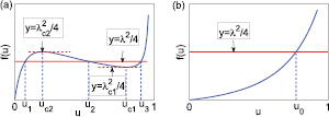
Figure 2. (a) The illustration for case (i):  . The blue solid line is the diagram of f . uc1 and uc2 are the local extreme points of f , and the two red dashed lines:
  and
and  are the tangents of f at uc1 and uc2. The red solid line represents line:
  (
( ) and this line intersects with the curve f (u) at u1, u2 and u3, which corresponds to the solutions of equation (28). (b) The illustration for case (ii):
  . The blue solid line and red dashed line also represent the diagram of f and line:
  , respectively. u0 is the intersection of these two lines, which corresponds to the unique solution of equation (28) in this case.
Download figure:
Standard image High-resolution imageThe eigenvalues of J(P) satisfy the equation  . Here
  and
and  represent the trace and determinant of J(P), respectively. Obviously,
  for all 0 < r < 1. With some calculation, we have
 ![$\det (J)=\left(1-{{r}^{2}}\right)\left[\left(2\beta +1\right){{r}^{2}}+1\right]{{f}^{\prime}}\left({{r}^{2}}\right)$](https://content.cld.iop.org/journals/1742-5468/2015/10/P10007/revision1/jstat519545ieqn115.gif) . For
. For  , we have
  and then
  . So the eigenvalues of J(P1) that satisfy the equation
  are both negative, showing that P1 is actually a stable node point of the system. For P2 and P3, we have
  and
and  thus indicating
  and
and  . Then J(P2) has two opposite-sign eigenvalues and J(P3) has two negative ones, indicating that the fixed point P2 is a saddle (unstable) point and P3 is a stable node point.
The stability of a fixed point decides whether it is an attracted state when t tends to infinity. For  , P1 is the only attractor and then the parameter r with an arbitrary initial value will tend to r1 as
  . For
. For  , two stable states P1 and P3 coexist. The parameter r will tend to r1 (or r3) when the initial state is close to P1 (or P3). For
  , the fixed point P3 becomes the only attractor and then r will tend to r3 with an arbitrary initial state.
This analysis actually indicates that there is a first-order phase transition of order parameter r from an incoherent state represented by P1 to a synchronized state represented by P3, where the values  and
and  correspond to the backward (
 ) and forward (
 ) critical coupling. The coupling intervals
  ,
,  and
and  correspond to the incoherent region, hysteresis region and synchronized region, respectively.
Case (ii):  . In this case, we have
  for all
  . Then f monotonically increases in the interval [0, 1) (see figure 2(b)). For a given
  , equation (28) has only one solution, corresponding to the unique fixed point
  ) of equations (26) and (27). Using the same method presented in case (i), we conclude that P is a stable node point of this system. As P0 is the only global attractor of the system, parameter r(t) will tend to r0 as
  with an arbitrary initial state. From figure 2(b), we can see that r0 should gradually increase from 0 to 1 as λ varies from 0 to
  . There is not a nonzero critical point for the transition from the incoherent state to the synchronized state. In other words, we say that the transition is continuous and the critical coupling point
  is zero.
The above results show that the synchronization phase transitions of the system depend on the width of perturbation distribution  . Small perturbations of frequencies (
 ) do not change the first-order synchronization transition of the original model in section 2, while large perturbations of frequencies weaken the degree-frequency correlation and then lead to a continuous synchronization transition. Besides, as
  , the model in this section described by equations (14) and (15) should approximate to the model without perturbations described by equations (1) and (2). We check this conclusion in the following. First, it is easy to check that
  and
and  . Then we have
  , which is just the forward critical coupling
  of the model in section 2. For uc1, we have
  as
as  , here
  is a function of β. Then we have
  , which is actually the backward critical coupling
  of the model described by equations (1) and (2). Moreover, the critical value of r as
  is
is  and
and  , which are just the same as the results of the model in section 2. The agreement of these two models when perturbations tend to zero partly confirms the validity of the method we used.
All of the results described above are obtained by analyzing the reduced ODE system governed by equations (26) and (27), and are therefore subject to the restrictions described therein. It is reasonable to ask if these results agree with the dynamics of the original system given in equations (14) and (15). To check this, a series of direct simulations of equations (14) and (15) using the fourth-order Runge–Kutta numerical integration are performed in the following.
Figure 3 presents the time evolutions of parameter r for different values of  and λ. The blue solid lines stand for the numerical simulations from the original model given in equations (14) and (15) with
  , while the red dashed lines are the analytical solutions obtained from equations (26) and (27). We fix
  and then we have
  . We choose two typical values of
  , 0.5 and 2.5 which correspond to case (i) and case (ii), respectively. Two different values of λ are chosen for each
  to stand for the weak coupling case and the strong coupling case. As we can see, the simulation results and the analytical solutions fit extremely well in all the four pictures, indicating that the reduced ODE system governed by equations (26) and (27) can quite precisely describe the time evolution of the order parameter r as N is large.

Figure 3. Time evolutions of r for  with different
  and λ. (a)
  ; (b)
; (b)  ; (c)
; (c)  ; (d)
; (d)  . The blue solid lines stand for direct simulations of the original model given by equations (14) and (15), and the red dashed lines stand for analytical solutions from the reduced equations given by equations (26) and (27). Network sizes are set as
  .
.
Download figure:
Standard image High-resolution imageFigure 4 shows the phase transition diagrams of the order parameter r. The parameter β here is set to be 10. The upper two figures are the simulation results of r versus coupling λ for  (figure 4(a)) and
  (figure 4(b)). For comparison, the lower two figures present the analytical solutions of r versus λ solved from equation (28). Figure 4(a) clearly shows a sharp jump of r and a hysteresis region between the forward and backward diagrams, which verify the existence of the first-order transition. The backward and forward processes in figure 4(b) coincide completely, showing that phase transition is actually continuous. Analytical results in figure 4(c) and (d) agree with corresponding simulations in figures 4(a) and (b). The backward and forward critical coupling obtained from the simulation in figure 4(a) is
  and
and  . They are quite close to the analytical results presented in figure 4(c), where
  and
and  .
.

Figure 4. (a), (b) Forward and backward synchronization diagrams r versus λ from direct simulation of equations (14) and (15) with  ,
,  ,
,  and 1.5. (c), (d) Synchronization parameter r versus λ given by analytical solutions of equation (28) for
  ,
,  and 1.5. The solid blue line and dashed red line in (c) stand for the stable and unstable branches of r, respectively.
Download figure:
Standard image High-resolution imageFor  , it has been shown that there is a first-order phase transition which is labeled by the two inconsistent critical couplings
  ,
,  and the existence of the hysteresis region. We are interested in how the value of critical coupling and the width of hysteresis depend on
  . To do this, we solve equation (32) for a fixed β and each
  to get the roots uc1 and uc2. Then we have
  and
and  . Figure 5(a) presents the values of
  and
and  for
for  when
when  varies from 0 to
  . We can see
  slowly increases with
  while
while  increases much faster until, at
  , the two lines overlap. The
  plane is then divided into three regions—the synchronized region (blue), hysteresis region (yellow) and incoherent region (purple). Figure 5(b) shows the hysteresis width
  as a function of
  . Here we can see it shows a descending trend starting from a certain level at
  and ending with
  at
at  .
.

Figure 5. (a) Phase space with critical couplings  and
and  versus
  for
for  dividing the phase space into incoherent, hysteresis and synchronized regions. (b) The hysteresis width
  versus
  .
.
Download figure:
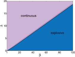
Standard image High-resolution imageFinally, we want to show how the parameter  and β codetermine the order of the phase transition of the system. We plot
  as a function of β from 1 to 100 in figure 6. Then the phase diagram is divided into two parts. In the upper part where
  , the phase transition is continuous while in the lower part where
  , transition is first-order (explosive). We can see that the boundary
  looks like a straight line. In fact, when
  ,
,  , and then by equation (32) we have
  . We plot
  as a dashed line in this figure and we can see that the two lines are quite close to each other.
Figure 6. The types of phase transitions of the system with different  and β. The boundary curve
  versus β separates the phase space into continuous and explosive regions. The dashed line stands for
  which is the asymptote of the curve
  as β is large.
Download figure:
Standard image High-resolution image
4. Conclusions and discussion
In this paper, we have analyzed ES on star graphs. Using the Ott–Antonsen ansatz, we first established a two-dimensional reduced system that can describe the evolution of the global behavior of the oscillators. We studied the dynamical behavior of this reduced system and showed that the phase transition from incoherence to synchronization is actually discontinuous. We also presented direct simulations of the original model and compared them to analytical results solved from the reduced system, and showed they have a good agreement. Then, we extended our model studied to a more general case where there are random perturbations to the frequencies of leaf nodes. We studied how the type of synchronization transition is decided by the perturbation strength  and the frequency of hub β. The results showed that for small perturbations the synchronization phase transition is still discontinuous while for large perturbations the transition becomes continuous.
Our works have completely solved the ES of Kuramoto oscillators on star graphs and have uncovered the intrinsic mathematical mechanism behind the first-order transition. For the SF network with tree-like structure, the modified model in section 3 can roughly describe the dynamic of the oscillators of star components. Then the results in this section can partly explain the mechanism of ES in this kind of network. Although it is still hard to completely solve the puzzle of ES on general SF networks, our work is still of important value in understanding the explosive phase transitions in large ensembles of coupled units, and moreover, it also points out some feasible directions and provides inspiration for a deeper investigation in the future.
Acknowledgments
This work is supported by the Major Program of National Natural Science Foundation of China (11290141), NSFC (11201018) and the international cooperation project no. 2010DFR00700.