

Abstract
Achieving atmospheric flight on Mars is challenging due to the low density of the Martian atmosphere. Aerodynamic forces are proportional to the atmospheric density, which limits the use of conventional aircraft designs on Mars. Here, we show using numerical simulations that a flapping wing robot can fly on Mars via bioinspired dynamic scaling. Trimmed, hovering flight is possible in a simulated Martian environment when dynamic similarity with insects on earth is achieved by preserving the relevant dimensionless parameters while scaling up the wings three to four times its normal size. The analysis is performed using a well-validated 2D Navier–Stokes equation solver, coupled to a 3D flight dynamics model to simulate free flight. The majority of power required is due to the inertia of the wing because of the ultra-low density. The inertial flap power can be substantially reduced through the use of a torsional spring. The minimum total power consumption is 188 W kg−1 when the torsional spring is driven at its natural frequency.
Export citation and abstract BibTeX RIS
1. Introduction
There are numerous challenges associated with flying on Mars. The challenge of flying in an ultra-low density environment can be summarized by the force balance between the wing lift L and weight W in equilibrium flight, expressed as
where CL is the lift coefficient, g and ρ are the Martian gravitational acceleration and atmospheric density, U is the free stream velocity, m is the vehicle mass, and S is planform area of both wings. Although the Martian g is about one-third of the acceleration on Earth, the average Martian atmospheric density is only 1.3% of the air density on Earth [1, 2]. Aerodynamic forces are proportional to the ambient fluid density, implying that conventional flight vehicle designs generate insufficient lift on Mars at subsonic cruise velocities. Another consequence of the low density is that the operational Reynolds number (Re) of small flight vehicles is of the order of O(102) to O(103) [1, 2]. The dynamic viscosity coefficient of the Martian atmosphere is 1.5 × 10⁻⁵ kg (m · s)−1 [3], similar to the value on Earth (1.8 × 10⁻⁵ kg (m · s)−1). In these low Reynolds number regimes, the lift coefficients of traditional fixed wing aircraft are significantly reduced [4]. To compensate for the reduced lift coefficient, all conventional aircraft designs must fly faster (higher U) or with a much lower wing loading (mg S−1). The near absence of oxygen in the Martian atmosphere prevents the use of air-breathing propulsion. Moreover, high take-off and cruise velocities pose significant operational challenges for air vehicle launch and recovery, as well as potentially complicating mission tasks. Take-offs and landings without any infrastructure will either require a hover-capable flyer or support equipment such as catapults, parachutes, or nets.
Several intriguing aerial vehicle concepts have been proposed to overcome the challenges associated with flying on Mars. Liu et al [5] provide a comprehensive review of these proposed designs. The aerial regional-scale environmental surveyor (ARES) was a rocket-powered, robotic airplane platform to aid the NASA Mars Exploration Program [6]. The prototype was designed to fly at Martian altitudes between 1 and 2 km. However, the ARES could not land on Mars' surface, and the concept was abandoned in favor of an orbiting surveyor. To explicitly tackle the issue of the low-density atmosphere, freely falling concepts and Mars balloons have also been proposed [5]. Additionally, NASA's Jet Propulsion Laboratory has considered a Mars Helicopter [5, 7, 8].
Bioinspired solutions for lift generation provide another set of Mars flight vehicle designs. For decades, the aerodynamics of insect flight remained inexplicable. A well-known example is the myth that bumblebees cannot fly according to classical aerodynamic theories [9]. Subsequent findings on unsteady lift production mechanisms [10–14] have enhanced our understanding of insect flight [4]. Insects rely on these unsteady aerodynamic mechanisms to produce high CL values [4] in low Re environments, such as the Martian atmosphere. Previous bioinspired concepts include the Entomopter, which is a flapping wing vehicle that uses a blown wing concept for lift enhancement, and the Solid State Aircraft, which is a solar-powered ornithopter [5]. However, both of these concepts suffer from the adverse effects of scaling up the entire vehicle in an effort to increase wing area. When the wing length scale l doubles to 2l, the wing area quadruples to 4l2, but the volume increases by 8l3. As illustrated in equation (1), the lift increases with the wing area by 4l2, insufficient to offset the weight increase of 8l3. Without a significant reduction in structural material density, a substantial technological challenge, the vehicle weight will likewise increase enough to make it improbable that these vehicles could fly on Mars. Moreover, the analysis of the Entomopter was based on simplified aerodynamic models, not including all the unsteady low Re lift production mechanisms. They were forced to augment lift production with the blown wing in order to achieve the large lift coefficients which are routinely achieved by insect-style flapping wings [4].
One of the complexities associated with studying insect flight and developing bioinspired micro-air vehicles (MAVs) is the number of morphological, kinematic, and aero/structural/dynamic parameters involved. The vast amount of data available on flapping wing insects such as bumblebees, hawkmoths, fruit flies, dragonflies, etc provides several potential starting points for a bioinspired flapping wing MAV. Rather than exploring the entire design space, we use dynamic similarity as a guideline to test the hypothesis that a bioinspired Mars flight vehicle can fly on Mars. We consider the bumblebee as a starting point for the design. The primary reason for this choice comes from the observation that the wing-to-body mass ratio of bumblebees is only 0.52% [15]. A significant increase in the wing area increases the total mass by only a fraction. By contrast, the lowest wing to total mass ratios in aircraft are typically 10% for large cargo aircraft such as the Boeing 747 [16]. Furthermore, a bumblebee's ability to hover and operate at high forward speeds with heavy payloads makes it a particularly attractive candidate for biomimicry since this feature aligns with the design goals of reconnaissance MAVs in general. That said, the scope of this study is limited to testing the hypothesis that a bioinspired hover solution exists when considering the coupled unsteady aerodynamics and flight dynamics. Since this is a question that has not been answered before, we believe that testing the existence of a bioinspired hover solution on Mars would be an appropriate first step before optimizing the performance.
The objective of this study is to investigate the aerodynamic performance of a bumblebee-inspired flapping wing vehicle in Martian atmospheric conditions. There are multiple methods with which to accomplish this analysis. One potential method is through quasi-steady models. Although the nature of flapping wings is inherently an unsteady aerodynamic problem, there has been much success in modeling the physics with quasi-steady models. For example, Lentink and Dickinson [17] showed that quasi-steady rotational accelerations can play a more important role compared to unsteady accelerations. Additionally, the experimental work of Usherwood and Ellington [18, 19] showed that the lift generated in the translational phase, as modeled by quasi-steady aerodynamics, is sufficiently high to balance weight in hover. Similarly, there are well validated theoretical models based on quasi-steady assumptions such as the blade element analysis [20] and the lifting line model [21] which can reasonably predict and model the forces produced by insect-like vehicles. However, it has been shown in our previous work [22] that wing-wake interaction, a nonlinear, unsteady aerodynamic effect, has a significant impact on the lift production, power required, and the flight dynamics. This leads us to use a Navier–Stokes (NS) solver which can accurately model this unsteady effect and therefore provide more accurate predictions of the vehicle's flight dynamics.
With this in mind, the study employs the NS equations to solve for the flow around the wings of a bioinspired Mars MAV and properly account for unsteady lift enhancement mechanisms, including delayed stall, wake-capture, rotational lift, and added mass effects. Additional unsteady mechanisms such as clap-and-fling and Wagner's effect can play a role but are of less importance in this study. All relevant dimensionless parameters are preserved to benefit from the high lift coefficients produced by insects on Earth. The NS solver is tightly integrated with a flight dynamics solver to ensure that the resulting wing design produces sufficient lift to sustain the total weight of the flyer in hovering free flight. The understanding of the role of unsteady aerodynamic mechanisms in Martian conditions can help the development and validation of quasi-steady flapping wing aerodynamics models for Martian flight in the future. The wing size and flapping frequency are varied to assess their effects on the resulting lift and power. Our results show that the natural bumblebee cannot sustain its weight in hover in the rarefied atmosphere on Mars. However, if we consider a so-called 'MarsBee', a hybrid bumblebee with larger wings that are scaled in all dimensions by a factor of n, ranging from 2 to 4.5, the resulting lift is sufficiently high to sustain its weight. This sufficient lift is achieved primarily by the enlarged wings which have four to twenty times the planform area of the Earth bumblebee wings.
It is important to note that only the aerodynamics and the free flight dynamics are considered in this study without any consideration for actuator dynamics or added actuator mass. The wing weight is properly scaled when a larger wing is considered with the assumption that the scaled wing is the same constituent material as the baseline bumblebee wing. The body mass is kept as a constant. Despite the recent advancements in material science, developing an autonomously flying bee-scale robotic flyer is still a challenge even on Earth. This study addresses the question of whether or not the flapping wing motion generates sufficient lift to sustain the weight of a wing-body configuration. Only after this fundamental question is positively answered can one consider developing a flapping wing robotic flyer and other components such as controllers, sensors, and power sources to actuate and sustain the motion. Additionally, this study is a prerequisite for optimizing the parameter design space, such as the wing kinematics, wing size, or adding power-saving devices, etc. The results of this investigation pave the way for system optimization and studying the effects of features such as wing flexibility as topics of future research.
2. Model and methods
2.1. Ensuring that lift balances weight through bioinspired dynamic scaling
To achieve hover on Mars, in addition to scaling up the wing, the flapping wing motion must be adjusted to offset the reduced density (ρmars ≈ 0.013ρearth) and reduced gravity (gmars ≈ 0.38gearth). Equation (1) can be rewritten in terms of the reference velocity U = 2πfΦR , where f is the sinusoidal flapping frequency in Hz, Φ is the half peak-to-peak flapping amplitude in radians, and R is the span of a single wing in meters (figure 1). This substitution results in
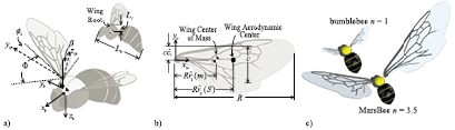
Figure 1. Schematic illustration of the key parameters for (a) the body and (b) the wing for (c) a bumblebee (n = 1) and a MarsBee with enlarged wing area (n = 3.5). The wing parameters are determined by considering the wing to be a composite of the fore-and hindwings, as calculated by Ellington [23].
Download figure:
Standard image High-resolution imageEquation (2) demonstrates that scaling the flapping frequency, flapping amplitude, or wing size can increase the lift.
We begin by quantifying the impacts that the reference wing tip velocity U ~ fΦ and the wing area S have on the resulting lift L. This can be expressed by introducing scaling parameter n for wing scaling, j for frequency scaling, and p for stroke amplitude scaling into equation (2), resulting in

where wing length R = nR0, mean chord c = nc0, stroke frequency f = jf0, and stroke amplitude Φ = pΦ0. Equation (3) demonstrates that the most efficient way of achieving lift is by increasing the wing size, as done in this study, since L scales with n4.
More importantly, the lift coefficient CL is a function of four dimensionless parameters that are subject to change in this study while operating on Mars with enlarged wings. Specifically we see that CL = CL(Re,M,k,α) [4, 24], where Re is the Reynolds number, M is the Mach number, k is the reduced frequency, and α is the angle of attack, respectively. Additional dimensionless parameters such as aspect ratio AR [4], Rossby number Ro [17, 25], and wing area distribution  [26, 27] can impact the lift coefficient but remain constant as a function of the geometric scaling considered in this study. We seek to preserve dynamic similarity between flapping on Mars and on Earth to be reasonably assured that the flapping wings will experience the high CL produced by insects. Exploring additional kinematics, 3D effects, and flexibility effects will be left as future work and will require considering a broader set of dimensionless parameters to preserve a high lift coefficient in the Mars MAV design. The dimensionless quantities and their typical values for insects on Earth and Mars are shown in table 1. In table 1, µ is the dynamic viscosity of the fluid, a is the speed of sound, and Utip = 2πfΦR.
Table 1. Relevant dimensionless parameters and their values. BB stands for bumblebee. Note that the values for the bumblebee on earth are either derived from or directly reported by [15].
| Dimensionless quantity | Symbol | Definition | Typical value for insects [4] | Values for BB on earth [15] | Values for BB on mars |
|---|---|---|---|---|---|
| Angle of attack | α | α | ~45° | ~50° | ~50° |
| Reduced frequency (hover) | k |  |
0.2 < khover < 0.4 | 0.348 | 0.348 |
| Reynolds number | Re |  |
O(102–104) | 1.68 × 10³ | 1.63 × 10² |
| Wing tip Mach number | M |  |
M < 0.1 | 0.033 | 0.3 |
Equations (2) and (3) and table 1 show that determining a dynamically similar hover solution is not trivial. The first constraint that must be considered is the effect of the flapping amplitude on the reduced frequency. Since AR is unchanged despite wing scaling (as the wing is scaled in all directions by the same factor n), the flapping amplitude Φ must remain similar to the biological bumblebee value in order to maintain an appropriate value for reduced frequency k in hover. It can be seen that Re is more sensitive to an increase in the wing size n as opposed to f or Φ. Specifically, Re scales with n2 since it is a product of both wing length R and chord length c. This would seem to suggest that wing scaling could quickly result in a Reynolds number that is no longer bioinspired. However, recall that Re also scales directly with the gas density  , which is significantly reduced in the case of Mars. As a result, Re can sustain a significant increase in n while maintaining a bioinspired value. As it turns out, the most influential driver of maintaining a dynamically similar solution is the wing tip Mach number. M scales equally with flapping frequency, amplitude, and wing size. However, refer back to equation (3) which demonstrates that frequency would need to be scaled by a factor of m2 to achieve the same amount of lift obtained with n4. Consequentially, if flapping frequency was chosen as the parameter to scale in order to produce the required lift, it would result in a Mach number that exceeds the typical range of insects. This means that the most efficient method of achieving lift and maintaining dynamic similarity is by scaling of the wing. This makes sense physically since scaling the wing size increases both the planform area S and the reference velocity (which affects the dynamic pressure due to a larger span R), both of which contribute to a higher lift (equation (1)). This is contrasted to scaling the frequency and flapping amplitude, which can only provide a higher reference velocity if they are increased.
Simply increasing the flapping frequency in equation (3) would not be a sufficient method for achieving lift on Mars. Specifically, the flapping frequency would need to increase by a factor of 6 to around 990 Hz to offset the lower Mars density and gravity. Although the Reynolds number and reduced frequency remain in the insect flight regime, the wing tip Mach number increases to around 0.3 (table 1). At this Mach number, compressibility effects can begin to become significant [28]. Also, it is unknown whether or not unsteady insect flight mechanisms can produce high lift coefficients at this value for M, which is beyond the scope of the present study.
Furthermore, as this study will eventually extend beyond hovering flight, it is important to also consider the relevant dimensionless parameters in forward flight. Both the forward flight reduced frequency  and the Strouhal number
  scale directly with the flapping frequency f. If a large frequency is required to achieve hover, then it is likely that these parameters could surpass their respective range typical of insect flight on earth, resulting in a solution that is not dynamically similar. These issues are not directly addressed in the current paper, but are under investigation in a separate work. A dynamically similar solution based on wing scaling is discussed in section 3.1.
2.2. Computational framework and governing equations
Flapping wing flight is characterized by unsteady flow with large vortical structures. To properly account for the unsteady lift enhancing mechanisms, the generation of large scale vortices [11] and their nonlinear interaction with the wing [12, 13] must be properly resolved by solving the NS equations. We tightly integrate the NS solver with a flight dynamics solver to create a flight simulator to determine the control inputs and other initial conditions required for the vehicle to hover on Mars. Of particular importance is the requirement that the lift balances the weight, where the wing weight scales with n3. For constant flapping frequency and amplitude, the resulting aerodynamic forces and moments scale with the wing scaling factor as n4, as shown in equation (3). We adjust the control parameters flapping amplitude Φ, stroke plane angle β, and flapping offset angle φo using the trimmer to find hover equilibrium. In order to maintain the Reynolds number and Mach number in the insect flight regime, we reduce the flapping frequency as discussed in section 3.1. Once a dynamically similar hover solution is established for each case, the resulting kinematics, aerodynamics, and power required are analyzed.
The computational framework demonstrated in figure 2 is based on our recent work [22] which couples a 2D NS equation solver to a nonlinear multi-body flight dynamics equation solver. Aerodynamic forces and moments on the flapping wings yield the body motion, which in turn affects the instantaneous fluid dynamics on the wings. To simulate free flight, the wing motion with respect to the wing root is prescribed by the wing kinematic parameters, while the body motion is simultaneously applied to the wing root. Therefore, the motion of the wing with respect to the air is a superposition of these two motions. The equations of motion are integrated at every time step. Hence, in free flight, the motion at each time step is a result of both the dictated wing kinematics and the body's free response. A detailed description and validation of the flight dynamics model and the coupling to the NS equation solver is described in our previous work [22]. A fully validated NS equation solver is used to calculate the velocity and pressure field around a flapping wing. NS equations are solved using an in-house 2D, structured, pressure-based finite volume solver [24, 29–32]. Remeshing is realized using the radial basis function interpolation scheme, shown to conserve good initial grid qualities and handle large wing motions and even deformations [4].
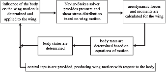
Figure 2. Computational framework based on previous work [22]. Flowchart describes the coupling between the NS and flight dynamics equations that occurs within a time step. The framework determines solutions for trimmed, hovering flight.
Download figure:
Standard image High-resolution image2.2.1. Wing kinematics
The wing kinematics are described using bio-inspired relations [33]. The flapping motion with respect to the wing root is a sinusoidal function of time t described by

where the flapping offset angle φo biases the flapping toward the ventral (+φo) or dorsal (−φo) side of the wing root. We prescribe a pitch angle θ as a rotation away from the vertical orientation in the stroke plane:
where the pitch amplitude is denoted by Θ. The timing of wing rotation is controlled by θφ, which can be positive for advanced rotation, zero for symmetric rotation, and negative for delayed rotation. Vertical deviation angle out of the stroke plane is not considered. Varying Cθ from ∞ to 0 transitions from a square wave to a sinusoidal wave. The pitching amplitude and pitch phasing angle are assumed to be Θ = 40° (refer to section 1 of the online supplemental material (stacks.iop.org/BB/13/046010/mmedia)) and θφ = 0.3, corresponding to advanced pitch rotation which is known to yield the highest lift [12, 35]. We set Cθ = 3.1, resulting in a modified square wave, as considered by other studies [14, 34]. The angle of attack at any instant is approximately α = π/2 − |θ|, although it also includes contributions from the body motion as well.
Motivated by the works of Badrya et al [35] and Faruque and Humbert [36], we select the stroke plane angle β, flapping amplitude Φ, and the flapping offset angle φo, as the three control inputs to actuate the three degree of freedom (3-DOF) system. Each control primarily affects the vertical, horizontal, and angular degree of freedom, respectively.
2.2.2. Aerodynamic modeling
We consider hover and hence any aerodynamic forces generated by the body can be neglected, since the body velocity is zero relative to the freestream. We only simulate a single wing, assuming left-right symmetry of the system confined to the 3-DOF pitch plane.
We directly solve the 2D incompressible NS equations
to determine the pressure and shear stress distributions on the wing. The velocity field V is normalized with the reference velocity U, or V* = V/U. Time is normalized by the flapping period (1/f), τ = f · t. Lengths are normalized by the mean wing chord c, and pressure is normalized per p* = p/ρU2. The Reynolds number is Re = Uc/ν, where ν is the kinematic viscosity. The reduced frequency in hover reduces to a geometric relationship that is governed by the stroke amplitude: k = πfc/U = c/(2Φ R).
R).
These equations are solved using a well-validated structured, finite-volume, pressure-based incompressible NS equation solver used extensively in flapping wing studies [29, 32]. Since the wing size, flapping frequency, and flapping amplitude change in each case, U, Re and k also change. For all bioinspired Mars MAV motions considered in this study, the resulting Reynolds number is in the range of 126 < Re < 187. In this Reynolds number regime, the fluid flow can be considered as laminar and the computational accuracy of the NS equation solver employed in this study is satisfactory [37]. Furthermore, 2D solutions have been previously shown to be a good approximation of the 3D flapping wing aerodynamics at Re = O(102) [37]. The main reason is that the effects of spanwise flow that seem to stabilize the LEVs [38] or LEV-tip-vortex interaction [39] on the overall aerodynamics are less important than at higher Reynolds numbers [13, 40]. Also, the characteristics of the LEVs in two-dimensions for plunging motions are representative of 3D flapping wings as long as the stroke-to-chord ratio is within the typical range of insects, i.e. around 4 to 5 [41], which we consider in this study. That said, 3D effects including the downwash distributions [42, 43] cannot completely be neglected and will be considered in the future.
The reduced frequency remains in the range of k = 0.29–0.32 due to variations in the flapping amplitude from case to case. The wing section is rectangular and modeled as a rigid flat plate with a 2% thickness to chord ratio (figure S1). The solver determines forces and moments at a rate of 480 time steps per flapping period. The wing is moved at each time step in accordance with the wing kinematics and body motion determined by the trimmer. The grid and additional computational setup are described in the appendix. The grid and time-step sensitivity studies were presented in an earlier work [44].
2.2.3. Dynamic interaction between the body and wing
We assume that the wing and body are rigid. The velocity bvcg and acceleration bacg of the body center of mass in the body frame are given by
where the leading subscripts b and w indicate that the variable is expressed in the body and wing frames, respectively. The rotation matrix  transforms vector components from the body to inertial frame and bωb/I is the angular velocity vector of the body with respect to the inertial frame, expressed in the body reference frame.
The velocity and acceleration of the wing consist of both the prescribed kinematics with respect to the body as well as contributions from the body motion itself. The resulting motion and orientation directly generates aerodynamic forces and moments. The velocity vector and acceleration of the wing aerodynamic center ac are given as

As indicated in figure 1(b), the aerodynamic center of the wing is the coordinate on the wing that is 25% chord from the leading edge and at the spanwise location of the center of the second moment of wing area (approximately 0.55R according to Ellington [23]). An equivalent expression can be derived for the wing's center of gravity wg. Detailed expressions for the angular rates, accelerations, and rotation matrices are provided in our earlier work [22].
To simulate free flight, the wing motion with respect to the wing root is prescribed by the control inputs (i.e. wing kinematic parameters), while the body motion is simultaneously applied to the wing root. Therefore, the motion of the wing with respect to the air is the superposition of these two motions. The 3D flapping is converted to a 2D plunge motion. The arc length of the second moment of wing area is set equal to the plunge amplitude ha = Φ R. The equations of motion are integrated at every time step. Therefore, in free flight, the motion at each time step is a result of both the dictated wing kinematics and the body's free response.
2.2.4. Equations of motion and determining equilibrium
With the mass of the wings included, the force and moment balance of the vehicle results in lengthy expressions, which are detailed in our previous work [22] and summarized here as
Here, the tilde over a vector quantity denotes a cross product and an over-dot represents the time derivative. FAero,w and MAero,w represent the aerodynamic contribution of the wing to forces and moments, respectively. In addition, g is the gravitational acceleration, mbody is the mass of the body, and Ib is the body inertia. Inertial properties of the bumblebee and other morphological parameters reported by Sun and Xiong [34] are used in this study and are summarized in table 2.
Table 2. Morphological parameters for the baseline bumblebee [34].
| Symbol | Description | Value | Symbol | Description | Value |
|---|---|---|---|---|---|
| mb | Mass of body | 175 mg | Iyy,b | Body moment of inertia (pitch) | 2.13 × 10⁻⁹ kg · m2 |
| mw | Nominal mass of wings | 0.91 mg | Lb | Body length | 18.61 mm |
| R | Length of a single wing | 13.2 mm | L1/Lb | Distance between CG & wing root | 0.21 |
| c | Mean chord of wing | 4 mm | f | Stroke frequency | 155 Hz |
 (S) (S) |
% span to 2nd moment of area | 55% | Ixx,w0 | Wing moment of inertia about wing root (pitch) | 1.48 × 10⁻¹² kg · m2 |
 (m) (m) |
% span to center of mass | 36% | Iyy,w0 | Moment of inertia about wing root (flap) | 3.07 × 10⁻¹¹ kg · m2 |
 (m) (m) |
% chord to center of mass | 25% | Izz,w0 | Moment of inertia about wing root (deviation) | 3.22 × 10⁻¹¹ kg · m2 |
| Ixz,wo | Product of inertia about wing root (deviation) | 2.18 × 10⁻¹² kg · m2 | |||
The system is tracked in state space form with a state vector
where it is restricted to motion in the x-z plane. In order to find the trimmed state at hover, we express equations (11) and (12) to highlight their dependence on the states and the control inputs as

where the elements of the system matrix, A, and the control matrix, B, are themselves nonlinear functions of the states and control inputs. We construct the A matrix numerically by perturbing each degree of freedom and using a central difference approximation to compare the system response with and without a perturbation. Each disturbance is modeled by moving the wing root with a prescribed motion that corresponds to the desired disturbance for three flapping cycles. During this time, the fluid's response to both the prescribed motion and flapping motion is computed and the surrounding wake is allowed to develop fully. The B matrix is obtained by perturbing each control in a similar fashion and determining its effect on the average system response.
In order to achieve hovering trim, we require  = mean([
 u w q]T) = 0, where the mean operator denotes the cycle averaged value. We utilize the trim method described by Badrya et al [35] and further detailed in our previous work [28] to find the necessary control inputs, i.e. Φ, φo, and β, and initial conditions, u0, w0, q0, and θ0 that place the system in equilibrium. Convergence is set such that
  < 1 × 10⁻² where the rate vector contains both accelerations (m s−2) and velocities (m s−1).
The detailed description of the free flight simulator and trim calculator as well as validation cases at fruit fly scales can be found in our previous work [22]. While we are able to validate our numerical free flight simulator against experimental results from flapping wing flyers on earth, we are not able to do the same for the Martian conditions. This is due to the fact that presently there is no accessible Martian atmosphere in which to conduct experimental flapping wing studies. However, when atmospheric conditions on Earth are used with bumblebee parameters, the flight simulator yields stability characteristics (figure 3) and power predictions that are in agreement with insect observations and values from previous studies. Figure 3 depicts the open loop poles of the longitudinal dynamics of bumblebees (BB) [34], drone flies (DF) [45, 46], and hawkmoths (HM) [46] reported in the literature compared to the values using our bumblebee numerical model with kinematics and morphological parameters set to match Sun and Xiong [34]. The qualitative response of all of these simulations is the same. Each insect has an unstable oscillatory mode and two stable subsidence modes. The magnitudes of the poles from our bumblebee simulation also compare favorably with the published NS simulations of similar insects.

Figure 3. Nondimensional open loop poles for bumblebee (BB) [34], drone fly (DF) [45, 46], and hawkmoth (HM) parameters [46].
Download figure:
Standard image High-resolution image2.3. Aerodynamic performance metrics
Operating in remote environments such as Mars dictates that power considerations are critical to vehicle design success. A flapping wing is actuated by imparting angular motion to the wing. Therefore, the power required is the product of the moment required to actuate the wing and the angular velocity of the wing. The required moment is simply the difference between the rate of change of angular momentum about the wing root (first term in equation (15)) and the aerodynamic moments (second term in equation (15))
Because the angular velocity components of the wing contain body rates the body motion affects the required wing power. At each simulation time step, the components of the moment are multiplied by the corresponding components of the angular velocity of the wing with respect to the body as
resulting in a time-history of power required. Note that this returns both positive and negative values. When Ppitch or Pflap is positive, power is required in order to achieve the desired wing motion. Because the atmosphere is so thin, and inertia dominates the power requirements, positive power typically occurs in portions of the stroke where the wing must be accelerated. Negative power typically occurs in the portions of the stroke where the wing decelerates. Many studies simply neglect negative power in their calculations [33, 47, 48], assuming that power is not expended during these portions of the stroke. We use the term positive power Ppos = mean( P(t) > 0) to refer to this definition.
We previously validated the power calculations for fruit fly motions [22]. The calculation of positive power required for several previous studies on bumblebees is provided in table 3 for a direct comparison to the power predicted from our simulations. Three calculations of power are included. The first is an estimate of power used by Dudley and Ellington [44] and Ellington [45], which sums the inertial, induced, and profile power based on observed kinematics. Engels et al [43] and Sun and Du [46] calculated the hovering power of a bumblebee using the same general method as equations (15) and (16) based on the forces and moments obtained from their solution to the 3D NS equations. Sun and Du [49] utilized 'idealized kinematics' with symmetric flapping. When we use the same kinematics, a slightly different trim solution results and the power differs by 9%. On the other hand, Engels et al [47] utilized observed kinematics of bumblebees in their 3D NS simulations. When we use observed kinematics provided in [50], our calculation of trim power agrees to within 3%. These favorable comparisons provide confidence in our simulation methodology.
Table 3. Summary of specific power for bumblebees reported in literature and current study.
| Ppos, W/kginsect | Calculation method | |
|---|---|---|
| Ellington [51] | 37.5 ± 1.5 | Estimated by summing induced, profile and inertial power, based on observed kinematics |
| Dudley and Ellington [48] | 55 ± 12 | |
| Sun and Du [49] | 56 | Directly calculated by 3D NS, using 'idealized' kinematics |
| Current study | 49.8 | Directly calculated by 2D NS, using 'idealized' kinematics from Du & Sun [49] |
| Engels et al [47] | 84 | Directly calculated by 3D NS, biomimetic kinematics |
| Current study | 81.3 | Directly calculated by 2D NS, biomimetic kinematics from Altshuler et al [50] |
Another way of treating power that we consider in this study is simply to directly average the negative and positive portions of the power required, Pave = mean(P(t)). This method assumes that the system can perfectly store the energy associated with negative power and fully utilize it in the parts of the stroke that require positive power. This method of calculating power provides an assessment of the minimum possible power required to fly, assuming a spring or other energy storage device is incorporated into the system to offset the large power consumption [48, 52, 53].
3. Results and discussion
3.1. Wing scaling and control parameters to achieve dynamically similar hovering
In order to justify the need to scale up the wings, we first test whether a standard bumblebee could fly on Mars. Using the flight simulator described in section 2, but with gravitational and atmospheric parameters that correspond to the Martian atmosphere, we solve for the control inputs that permit hovering flight on Mars. Per table 4, flight for a standard bumblebee (i.e. n = 1) in a Martian atmosphere requires a flapping amplitude of Φ = 366.3°. When the half peak-to-peak flapping amplitude exceeds 90°, the left and right wings touch each other, which is not physically permissible. Therefore, the wing kinematics and morphology of a standard bumblebee cannot generate sufficient lift on Mars because the Martian atmosphere is too thin.
Table 4. A summary of physical and flapping parameters for bumblebee flight on Earth and Mars, as well as Mars MAV flight on Mars. Results are based on our coupled NS-flight dynamics code. Note that bumblebee flight on Mars in characterized by an unphysical flapping amplitude as well as a reduced frequency that results in a non-dynamically similar solution. However, the dimensionless parameters for both Mars MAVs result in dynamically similar solutions, where n = 3.5 requires the least amount of power among Mars MAV solutions.
| Bumblebee on Earth | Bumblebee on Mars | Mars MAV on Mars, n = 2.5 | Mars MAV on Mars, n = 3.5 | |
|---|---|---|---|---|
| Wing size factor | 1 | 1 | 2.5 | 3.5 |
| Atmospheric density [kg m−3] | 1.225 | 1.55 × 10⁻² | 1.55 × 10⁻² | 1.55 × 10⁻² |
| Gravitational acceleration [m s−2] | 9.81 | 3.72 | 3.72 | 3.72 |
| Viscosity coefficient [kg (ms)−1] | 1.8 × 10⁻⁵ | 1.5 × 10⁻⁵ | 1.5 × 10⁻⁵ | 1.5 × 10⁻⁵ |
| Body mass [kg] | 1.75 × 10⁻⁴ | 1.75 × 10⁻⁴ | 1.75 × 10⁻⁴ | 1.75 × 10⁻⁴ |
| Total wing area [m2] | 1.06 × 10⁻⁴ | 1.06 × 10⁻⁴ | 6.60 × 10⁻⁴ | 1.29 × 10⁻³ |
| Mass of wings [kg] | 9.10 × 10⁻⁷ | 9.10 × 10⁻⁷ | 1.42 × 10⁻⁵ | 3.90 × 10⁻⁵ |
| Wing mass/body mass | 0.52% | 0.52% | 8.13% | 22.3% |
| Total mass [kg] | 1.75 × 10⁻⁴ | 1.75 × 10⁻⁴ | 1.88 × 10⁻⁴ | 2.13 × 10⁻⁴ |
| Total weight [mN] | 1.72 | 0.652 | 0.702 | 0.794 |
| Flapping amplitude [°] | 41.6 |
366 | 53.9 | 55.3 |
| Flapping frequency [Hz] | 155 | 155 | 114 | 63.1 |
| Reynolds number | 1439 | 340.6 | 127 | 141 |
| Wing tip Mach number | 0.028 | 0.33 | 0.05 | 0.03 |
| Aspect ratio | 3.3 | 3.3 | 3.3 | 3.3 |
| Angle of attack | 50° | 50° | 50° | 50° |
| Reduced frequency | 0.4054 | 0.048 | 0.323 | 0.315 |
| Power required [W] | 0.012 | 0.19 | 0.20 | 0.19 |
| Specific power required [W kg−1] | 68.6 | 1090 | 1090 | 901 |
| Flap amplitude less than 90°? | Yes | No | Yes | Yes |
aFlapping amplitude for bumblebee on earth using advanced rotation.
Figure 4 shows the control parameters that yield hover equilibrium on Mars. It can be seen that the resulting flapping amplitudes remain in a relatively small range (figure 4(a)). This is by design, resulting in a relatively consistent value for the reduced frequency in hover k = 1/(ΦAR). Recall that by consistently scaling up the chord and span by n, the aspect ratio AR is kept the same. Thus, the resulting k for the MarsBees ranges from 0.315 to 0.323 which is within the insect flight regime. The Reynolds number remains of the order of O(102) by reducing the flapping frequency as the wing size increases (figure 4(b)). The stroke plane angle β and the flapping offset angle φo are also provided, but their variation for different wing sizes is small. Although the wing's velocity is larger than on Earth and the speed of sound on Mars is approximately 72% of the speed of sound on Earth [2], the Mach number remains less than 0.09, indicating that the flow is incompressible and within the insect flight regime.

Figure 4. Control parameters required to hover on Mars for various wing sizes for (a) the flapping amplitude, (b) flapping frequency, (c) stroke plane angle, and (d) offset angle.
Download figure:
Standard image High-resolution imageTable 4 also shows the main parameters of realizable flapping motions for trimmed, hovering flight on Mars for a family of hybrid Mars MAVs (MarsBees) consisting of enlarged wings on a bee's body (figure 1(c)) with lift equal to total weight. When the chord and span of a standard Earth bumblebee wing are increased by factors of n = 2.5 and n = 3.5, i.e. the area is increased by corresponding factors of 6.25 and 12.25, sufficient lift can be generated that can offset the increased total weight. Despite the cubic increase in the wing weight, the total system weight increases only by 8% and 22%, respectively. This is again a benefit of the nominal bumblebee's small wing-to-body mass ratio. Note that in table 4, the bumblebee on earth simulation was performed using the same kinematics used in the MarsBee simulations (section 2.2.1). As a result of maintaining consistent kinematics across simulations, namely the use of advanced rotation, the flapping amplitude for the bumblebee on earth is lower than typically reported in literature. This is expected, as advanced rotation is reported to produce higher lift compared to the symmetric pitching typical of biological flapping motion [12, 35]. This reasoning also applies to the slight discrepancies between the dimensionless parameters presented in tables 1 and 4 for the bumblebee on earth.
Although we use the bumblebee parameters as a starting point in this study, we seek a bioinspired Mars flight design that falls within the insect flight regime, not necessarily constrained by the bumblebee regime. The larger wing of the bioinspired Mars MAV allows hover in the low density environment on Mars. However, the penalty associated with using such large wings is clearly seen in the power required to actuate them. From table 4, operating on Mars requires over 13 times the power to fly on Earth when considering the case where the wings are scaled by a factor of n = 3.5. Because of the ultra-low density in the Martian atmosphere, the resulting Reynolds number reduces to Re = O(102), which is an order of magnitude lower than the Earth bumblebee Reynolds number. The higher power required for the Mars flight vehicle compared to the bumblebee on Earth suggests that the performance may be further improved. Moreover, the reduced performance may be ascribed to the fact that the Mars flight vehicle operates at a reduced Reynolds number. Still, the resulting Reynolds number is within the insect flight regime and the resulting lift coefficient is sufficiently high such that the bioinspired Mars flight vehicle is able to sustain its own weight on Mars. The power required is further discussed in more detail in section 3.3.
3.2. Low Reynolds number aerodynamics on Mars
Figure 5 shows the lift histories for various wing sizes subject to the constraint of operating in trim on Mars. Each trace describes the average lift that is necessary to balance the weight on Mars for the wing size factor of n = 1 (bumblebee on Mars) and n = 2.5, 3.5 (bioinspired MAVs on Mars). The associated drag and wing kinematics are included in figure 5 as well. This figure also depicts the unsteady lift generation mechanisms that yield much higher lift coefficients than conventional airplane or helicopter designs at low Reynolds numbers [54]. Insects use unsteady lift production mechanisms, including the well-known mechanisms of delayed stall, rotational lift, added mass forces, and wing-wake interaction (or wake-capture) [4, 11–14] to fly. These unsteady lift generation mechanisms are the reason that the dynamically similar flapping wings can produce sufficient lift despite the low-Reynolds environment on Mars.
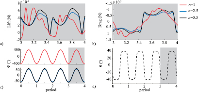
Figure 5. (a) Lift and (b) drag produced by a bee on Mars (n = 1) and two bioinspired Mars MAVs (n = 2.5 and n = 3.5) during the fourth and final flapping period. Corresponding (c) flapping and (d) pitching motions, where the flapping amplitude varies as a function of n while the pitching amplitude is the same for all values of n.
Download figure:
Standard image High-resolution imageThe lift time histories are qualitatively similar for n = 2.5 and 3.5 with the averaged lift being higher for n = 3.5 because the total weight is greater in trim. To simplify the discussion, we only compare the lift production mechanisms and vortex dynamics between n = 1 and 3.5 in this section. The corresponding vorticity contours are illustrated in figure 6 for n = 1 and 3.5. The wing is flapping from left to right with advanced rotation. The z-component of vorticity is positive into the page and it is normalized by U/c. The vorticity contours clearly identify the location and direction of the vortical structures relative to the wing. The leading-edge vortex generated in the current stroke is denoted by LEV1; the LEV shed in the previous stroke is labeled as LEV0, and so on. Trailing-edge vortices (TEVs) follow the same convention.

Figure 6. Unsteady vortex generation for (a) n = 1 where f = 155 Hz, Φ = 366.3° and (b) n = 3.5 where f = 63.1 Hz and Z = 55.3°. The unphysically large stroke amplitude in conjunction with the bumblebee's natural flapping frequency results in (a) flow structures and a lift history which are not exhibited by insects. However, the flow structures for the case of (b) n = 3.5 are similar to those for typical flapping flyers. Vorticity is normalized with U/c.
Download figure:
Standard image High-resolution imageThe first high-lift mechanism is wake-capture, which causes the large lift increment for n = 3.5 at the stroke ends τ = 0 and τ = 0.5. During this phase of the stroke, the wing encounters the LEV0 (figure 6(b) at τ = 0) that was shed during the previous half-stroke, enabling the wing to recover energy from the flow [30, 31]. In the case of n = 1, however, the vortex structures in the immediate vicinity of the wing are dominated by the TEV0 shed during wing rotation, which imparts downwash on the wing and delays lift production from wing-wake interaction with LEV0 until τ = 0 to 0.0625. This is reflected in figure 5(a), where no lift increment is seen at τ = 0 or τ = 0.5 for n = 1.
The second region of large lift generation for n = 3.5 occurs from τ = 0.125 to 0.35 in the first half-stroke and from τ = 0.625 to 0.85 in the second half-stroke (figure 5(a)). The lift in this region results from the stable LEV1 that forms during the translational phase of the stroke, hence it is termed translational lift [12]. The stable LEV1, which can be seen at τ = 0.25 and 0.375 for n = 3.5 in figure 6(b), significantly reduces the pressure behind the wing and increases the lift.
On the other hand, in the case of n = 1, two separate LEVs form in each half-stroke with a noticeable shedding event that results in the abrupt loss of lift immediately preceding and following τ = 0.25 in figure 5(a). The first LEV1a that forms can be seen at τ = 0.125 (figure 6(a)) associated with the second lift peak (figure 5(a)). The timing of this lift peak is earlier than the case of n = 3.5 because of the unphysically large flapping amplitude, yielding a relatively faster flapping motion. It is destabilized by interference from LEV0 and by the rapid growth of TEV1, leading to the separation of LEV1a around τ = 0.2. A new LEV1b can be seen forming at τ = 0.25, and it produces the third lift peak at τ = 0.3 in figure 6(a). This process is repeated in the second half stroke. Thus, for the n = 1 case, the translational force mechanism is the source of both peaks that are seen in figure 5(a) in each half stroke, with delayed contributions from wake-capture generating the first peak. The strength and size of the TEV0 is much larger for n = 1, which changes the overall flow field and prevents the LEV0 from interacting with the wing as described previously for the bioinspired Mars MAV configurations (n = 3.5).
The lift time history and the vortex dynamics for the bioinspired Mars MAV configuration at n = 3.5 resemble the insect flapping aerodynamics for hover with both wake capture and delayed stall lift peaks [4]. However, when n = 1, wake capture is delayed by the unphysically large flapping amplitude, and the delayed stall mechanism is characterized by two noticeable shedding events of the LEV. This discussion demonstrates that a bioinspired dynamic similar solution is promising and important to realize flying on Mars by flapping motion.
3.3. Power required to hover with larger wings
The time histories of flapping and pitching power required to hover on Mars are shown in figure 7 for various wing sizes. The time history of the flap power resembles a sinusoidal profile. The peak flap power varies with n. On the other hand, the pitch power is zero during the midstroke, when the pitch angle is held constant as shown in equation (16). At the ends of the strokes, the wing rapidly rotates, leading to large peaks. Since both flapping and pitching power are functions of multiple variables (e.g. wing speed, lift and drag coefficients, and wing size), we do not see a monotonic trend in the amplitudes of the pitch power. Additionally, both flapping and pitching power are less than zero for significant portions of the stroke. The flap and pitch power peaks are of approximately the same magnitude. However, the pitch power peaks are of much shorter duration.

Figure 7. Time histories of the (a) flap and (b) pitch power for different wing sizes n. The curves show that there is not a direct monotonic scaling between the wing size n and the power amplitude for either flapping or pitching. This is because the flapping and pitching power are functions of multiple variables, such as wing speed, lift and drag coefficients, and wing size.
Download figure:
Standard image High-resolution imageFigure 8 shows the inertial and aerodynamic contributions to the required flap and pitch power. Most significantly, in both the flapping and pitching power, the inertial contribution to power is approximately two orders of magnitude larger than the aerodynamic contribution to power. The moment of inertia increases with scale factor by n5, which significantly increases the inertial power. Also, the Martian air is so thin that the aerodynamic power is much lower than it is on Earth, all else being equal.

Figure 8. Power requirements for different wing sizes n = 2.5, 3.5 and 4.5. (a) Inertial flap power; (b) inertial pitch power; (c) aerodynamic flap power; (d) aerodynamic pitch power. The inertial power required is orders of magnitude larger than the resulting aerodynamic power for flapping wings on Mars. This is due to the ultra-low density of the atmosphere.
Download figure:
Standard image High-resolution imageFigure 9 depicts the pitch, flap, and total positive power, Ppos, for various wing sizes. Additionally, the average power, which is averaged over one cycle, is presented in figure 9. This is considered the ideal power because it assumes that all negative power can be stored and perfectly recovered, thus negating some, or all, of the positive power. In the Martian atmosphere, a bumblebee with nominal wings (n = 1) would require approximately 0.19 W to achieve hover (table 4), although we showed in section 3.1 that a physically impossible flapping amplitude is required to do so. On the other hand, increasing the wing size by a factor of n = 2.5–3.5 and reducing the flapping frequency will reduce the required power to approximately 0.17 W and 0.16 W respectively. Increasing the wing size further, however, causes an increase in the total power required. The specific power curve has a clear region where flight with minimum power is obtained between n = 3 and n = 4 for the given kinematics.

Figure 9. Specific power for different wing sizes n based on NS simulations, normalized by the total mass. (a) Positive power for pitch, flap, and total power. (b) Power comparison for positive power (with and without torsional springs) and the ideal case of average power, which assumes that all negative power can be stored and perfectly recovered. The power reduction with the torsional springs (see section 3.5) is ~80% for each case. This is a direct result of the springs operating at their resonance frequency and thus negating the inertial flap power required. The resulting power for the torsional spring cases is the sum of the aerodynamic flapping power plus the aerodynamic and inertial pitching power. Note how the positive spring power curve approaches the ideal case of the average power and is slightly more than the total pitching power due to the aerodynamic flap power required.
Download figure:
Standard image High-resolution image
3.4. Inertial cause of power required
The nonlinear trend in power with respect to a variation in the wing size n can be explained by considering the inertial contribution to the total power. As shown in figure 8, the inertial power is orders of magnitude greater than the aerodynamic power because of the ultra-low Martian density for both flap and pitch powers. As the wing size n varies, both the required flapping amplitude Φ and flapping frequency f change to achieve hover equilibrium as shown in figure 4.
The inertial flap power for a pair of wings can be found by inserting equation (2) in equation (16), yielding

where the moment of inertia of the wing scales as Iyy = Iyy,0n5 under a wing size variation n. The subscript 0 indicates the nominal wing size value.
On the other hand, the relationship between the flapping amplitude, frequency, and wing size, subject to the condition that the lift balances the weight, can be estimated from equation (1) as
where the wing area is S = 2Rc, and wing length and mean chord vary with n as R = R0n, c = c0n, and, again, U = 2πfΦ R.
R.
To dissect the influence of Φ and f on Pflap,inertial, we first hold Φ constant and adjust f to achieve equilibrium. Then we hold f constant and adjust Φ. Since we consider the same wing shape,  is also constant. Additionally, the change in the total weight is relatively small with respect to n as discussed before. Furthermore, our simulations indicate that the lift coefficient is close to CL = 1 for all cases. For simplicity, we define a parameter M = (mg/4π2
 )1/2 that is held constant in the following analysis.
When Φ is kept constant, the required flapping frequency becomes f = M/Φn2 from equation (18). Then equation (17) becomes
indicating that Pflap,inertial,Φ is inversely proportional to n. The effect of f on Pflap,inertial can be similarly determined as

which shows that Pflap,inertial,f is proportional to n. As the wing size increases, the flap amplitude contribution reduces. However, the flap frequency contribution to the inertial flap power increases with n. As a result, there is an optimal wing size as shown in figure 9. This is because both f and Φ have a similar order of contribution to produce lift that balances the weight (equation (18)). However, Pflap,inertial ~ f 3 whereas Pflap,inertial ~ Φ2 (equation (17)), yielding the qualitatively different influences of the flap amplitude and frequency on the inertial flap power. The pitch power trends are qualitatively similar.
For illustrative purposes, scaling the wing up by n = 3.5 in each dimension is equivalent to a bumblebee using the forewing from a cicada. Operating such a large wing is necessary to compensate for the low density environment on Mars. However, as previously mentioned, the penalty associated with using such large wings is clearly seen in the power required to actuate them (table 4). There are methods for optimizing the wing kinematics [55] such that power is reduced, as well as many practical methods for eliminating sources of power in flapping wing motions, as discussed in the following section.
3.5. Eliminating inertial flap power with torsional springs
In order to reduce the total power required we propose another benefit of using the flapping motion as a propulsive mechanism on Mars. We place a torsional spring (patent pending) at the root of each wing to temporarily store otherwise wasted energy and reduce the overall inertial power when driven at resonance. The effects of a spring on the flapping wing motion are modeled by a second order ordinary differential equation as

in the wing frame, where  is the wing root (flap) moment of inertia, Taero is the aerodynamic torque, kT is the angular spring constant, Treq is the torque required from the forcing function, and
  is the instantaneous flapping angle of the wing. The dot and double dot represent the first and second time derivative, respectively. Equation (21) relates the flapping wing kinematics to the material properties of the spring and the forcing function required to impose the desired motion φ given by the trimmed solution, e.g. figure 4(a).
According to equation (4), the flapping motion is sinusoidal and can therefore be written as  . When
  is and
  are substituted into (21), the result is
We choose the spring constant to align the undamped natural frequency fn with the flapping frequency
When equation (23) is substituted into equation (22) the inertial and spring terms cancel out, resulting in Treq = Taero. Thus, when the torsional spring is driven at its resonant frequency, the required torque for the flapping motion is only comprised of the aerodynamic torque, which is orders of magnitude lower than the inertial torque (figure 8). As a result, the total power required reduces substantially. This method takes advantage of the ultra-low density environment on Mars and negates the increased inertial flap power required due to wing scaling. Where the low density was initially an obstacle to overcome, it is now a benefit when considering torsional springs placed at the wing roots.
Note that a similar, closed form analytical expression is not derived for the inertial pitching component of the total power required. This is due to the fact that the pitch motion is described in terms of a hyperbolic tangent function, as seen in equation (5). This limits the ability to express the derivatives required for writing equation (16) in a concise analytical form. Additionally, for both the aerodynamic flapping and pitching power components, we are unable to rewrite the Navier–Stokes equations in a way that captures the all of the flapping/pitching motion of the wing, as well as the body motion. However, it still stands that the most dominant source of power is the inertial flap power, as demonstrated by figures 8 and 9(a). This means that the expression for the inertial flap power in equation (17) captures the important kinematic/morphological parameters that drive the overall power required.
Figure 9(b) compares the flapping power required for MarsBees with wings that have been scaled by a factor of 2 < n < 4.5 with and without torsional springs. The power required for the simulations which include the springs is composed of the aerodynamic flapping power and both the inertial and aerodynamic pitching power. For the case where n = 3.5, the total power required is reduced by 79% from 0.19 W to 0.04 W when torsional springs are placed at the wing roots. Note that the resulting power of 0.04 W is now only 3.3 times the power required for a natural bumblebee to fly on Earth, which is 0.012 W (table 4).
Considering the specific power for the case of n = 3.5 on Mars, the total specific power for wings without torsional springs is 901 W kg−1 (table 4). This can be compared to the n = 3.5 case with the torsional springs which has a total specific power of 188 W kg−1, and the nominal earth bumblebee specific power of 68.6 W kg−1. As a measure of ideal flight endurance, where the entire body mass is comprised of a lithium-ion battery with a specific energy of 243 Wh kg−1 (Panasonic NCR18650B lithium-ion battery), the flight times for the case of n = 3.5 are 16 min without the springs and 78 min with the springs. This ideal scenario assumes a 100% efficiency for the transmission of power from the battery to the MAV's wings. Even in the baseline case without the springs, the endurance time is similar to that predicted by the Mars Scout Helicopter, which is approximately 90 seconds [7].
4. Concluding remarks
The objective of this study is to investigate the aerodynamic performance of a bumblebee in Martian atmospheric conditions. The Navier–Stokes equations are solved for the flow around the bumblebee to properly account for the unsteady lift enhancement mechanisms. The wing size and flapping frequency are varied to assess their effects on the resulting lift and power. Our results show that the bumblebee cannot sustain its weight in hover in Mars' low-density atmosphere, even with its lower gravitational acceleration. However, we show using numerical simulations that a bumblebee inspired flapping wing robot can fly on Mars via bioinspired dynamic scaling. Trimmed, hovering flight is possible in a simulated Martian environment when dynamic similarity is achieved by preserving all relevant dimensionless parameters. Results show that a significant increase in the wing area S changes the total mass m by only a fraction, indicating that the wing loading can be made much lower than other Martian aerial concepts such as the Entomopter, or even a bumblebee. Our results suggest that when the bumblebee wing is enlarged, for example, by a factor of 3.5, a flapping motion with an amplitude of 55.3° and frequency 63.1 Hz can generate sufficient lift to sustain the increased weight on Mars. The penalty for increasing the wing size, however is a significant increase in the power required from approximately 69 W kg−1 to 900 W kg−1. However, if a torsional spring is placed at the wing root, the power required can be reduced by 80% to a value of approximately 188 W kg−1. It can be further reduced by the implementation of passive pitching.
Although we solve the Navier–Stokes equations, the considered flow is 2D. Also, the present work is limited to a few design parameters governing the kinematics and morphological parameters. Furthermore, the power consumption even with the addition of a torsional spring is still quite high compared with insect flight on Earth in terms of muscle mass-specific power. Developing a physical model will be challenging. That said, the presented design can be further improved through optimization studies. For example, the use of flexible wings with non-uniform and anisotropic structural properties like insect wings can further reduce the power consumption. Future work will include investigations into materials, batteries, and actuators.
Acknowledgments
This work was in part supported by the NASA Innovative Advanced Concepts program under the grant 80NSSC18K0870 and partly by the University of Alabama in Huntsville through supplemental research funding to CK. JB's work is supported by the US Army Advanced Civil Schooling program. JP is supported by the Alabama Space Grant Consortium Fellowship, NASA Training Grant NNX15AJ18H. CK thanks Bryan Mesmer of the University of Alabama in Huntsville for the fruitful discussions on the system analysis.