

Abstract
New metrics and evidence are presented that support a linkage between rapid Arctic warming, relative to Northern hemisphere mid-latitudes, and more frequent high-amplitude (wavy) jet-stream configurations that favor persistent weather patterns. We find robust relationships among seasonal and regional patterns of weaker poleward thickness gradients, weaker zonal upper-level winds, and a more meridional flow direction. These results suggest that as the Arctic continues to warm faster than elsewhere in response to rising greenhouse-gas concentrations, the frequency of extreme weather events caused by persistent jet-stream patterns will increase.
Export citation and abstract BibTeX RIS

Content from this work may be used under the terms of the Creative Commons Attribution 3.0 licence. Any further distribution of this work must maintain attribution to the author(s) and the title of the work, journal citation and DOI.
This paper builds on the proposed linkage between Arctic amplification (AA)—defined here as the enhanced sensitivity of Arctic temperature change relative to mid-latitude regions—and changes in the large-scale, upper-level flow in mid-latitudes [1, 2]. Widespread Arctic change continues to intensify, as evidenced by continued loss of Arctic sea ice [3]; decreasing mass of Greenland's ice sheet [4], rapid decline of snow cover on Northern hemisphere continents during early summer [5], and the continued rapid warming of the Arctic relative to mid-latitudes. While these events are driven by AA, they also amplify it: melting ice and snow expose the dark surfaces beneath, which reduces the surface albedo, further enhances the absorption of insolation, and exacerbates melting. Expanding ice-free areas in the Arctic Ocean also lead to additional evaporation that augments warming and Arctic precipitation [6].
Traditionally AA is measured as the change in surface air temperature in the Arctic relative to either the Northern hemisphere or the globe [7]. It arises owing to a variety of factors, including the loss of sea-ice and snow, increased water vapor, a thinner and more fractured ice cover, and differences between the Arctic and lower latitudes in the behavior of lapse-rate and radiative feedbacks [8–13]. Here we do not address the relative importance of various factors causing AA, but it is clear from the height-latitude anomalies of air temperature, geopotential, and zonal wind (figure 1) that AA results in large part from near-surface heating, although contributions from poleward heat transport may also play a role [14].

Figure 1. Annual-mean anomalies in air temperature (left), geopotential (middle), and zonal winds (right) during 1995–2013 relative to 1981–2010 for 40–80°N and 1000–250 hPa. Data were obtained from the NCEP/NCAR Reanalysis at http://www.esrl.noaa.gov/psd/.
Download figure:
Standard image High-resolution imageSeasonal time series and trends in AA based on two metrics and varying initial years are presented in figure 2. The more traditional method of assessing AA is to subtract changes in near-surface (1000 hPa) air temperature anomalies in mid-latitudes (60–30°N) from those in the Arctic (left side of figure 2). A positive value of AA indicates that the Arctic is warming faster than mid-latitudes. Both the time series and progressive 15 year trends (figure 2, bottom) indicate an increasingly positive AA in all seasons, particularly in fall and winter, in agreement with previous analyses [8]. Starting in the 1990s, coincident with an accelerated decline in Arctic sea-ice extent [3], AA values and trends became positive in all four seasons for the first time since the beginning of the modern data record in the late 1940s, illustrating the Arctic's enhanced sensitivity to global warming.
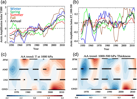
Figure 2. Arctic amplification seasonal time series (a), (b) and trends (c), (d) based on two metrics: (left) differences in 1000 hPa temperature anomalies (relative to 1948–2013 mean, °C) between the Arctic (70–90°N) and mid-latitudes (30–60°N); (right) differences in 1000–500 hPa thickness anomalies (percent of mean for each zone) between the two zones. Contoured colors in c,d indicate moving 15 year trends (C/decade for T1000 and percent of mean per decade) for each season. The x-axis indicates the ending year of each 15 year period between 1949 and 2013, and asterisks indicate ending year of periods with significant trends (confidence >95%, assessed using an F-test goodness of fit). Data were obtained from the NCEP/NCAR Reanalysis at http://www.esrl.noaa.gov/psd/.
Download figure:
Standard image High-resolution imageThe right side of figure 2 presents an alternative metric for AA based on the difference in the 1000–500 hPa thickness change in the Arctic relative to that in mid-latitudes (same zones as for the traditional method). Arguably the thickness difference is more relevant for assessing the effects of AA on the large-scale circulation, as it represents differences in warming over a deeper layer of the atmosphere that should more directly influence winds at upper levels. Several recent autumns have exhibited strong warming anomalies in some mid-latitude areas, contributing to the weakened positive trend after 2007. It is important to note the recent emergence of the signal of AA from the noise of natural variability: since ∼1995 near the surface and since ∼2000 in the lower troposphere. This short period presents a substantial challenge to the detection of robust signals of atmospheric response amid the noise of natural variability [15, 16]. Thus for this study we define the period from 1995 to 2013 as the 'AA era.' While this demarcation is consistent with previous studies [17], we also investigate the effects of choosing different commencement years on detecting changes in the frequency of high-amplitude jet-stream configurations.
The following linkage between AA and mid-latitude weather patterns has been hypothesized [1]. Increasing AA weakens the poleward temperature gradient—a fundamental driver of zonal winds in upper levels of the atmosphere—which causes zonal winds to decrease, following the thermal wind relationship [18]. A weaker poleward temperature gradient is also a signature of the negative phase of the so-called Arctic oscillation/Northern annular mode (AO/NAM), in which weaker zonal winds are associated with a tendency for a more meridional flow, blocking, and a variety of extreme weather events in much of the extratropics [19]. Disproportionate Arctic warming and sea-ice loss favor a negative AO/NAM aloft [1, 2, 20, 21] and a Northward migration of ridges in the upper-level flow [1], further contributing to an increased meridional pattern. As the wave amplitude and/or frequency of amplified flow regimes increases, the incidence of blocking becomes more likely [2], which reduces the Eastward propagation speed of the pattern. Consequently, the associated weather systems persist longer in a particular area. Extreme weather events caused by prolonged weather conditions (such as cold spells, stormy periods, heat waves, and droughts), therefore, should also become more likely, as illustrated by recent studies linking these events to high-amplitude planetary waves [22–24].
Because AA is strongest in fall and winter (figure 2), the atmospheric response is expected to be largest and observed first in these seasons. Results corroborate this expectation [1], showing a marked reduction in the poleward thickness gradient and weaker zonal winds at 500 hPa during fall (OND) and winter (JFM) since 1979 over the North America/North Atlantic study region. Others find statistically significant decreases in zonal-mean zonal winds in the fall but not in winter [15].
Marked spatial and seasonal variability in the changing poleward thickness gradient dictates patterns of change in zonal winds. While hemisphere-mean, mid-latitude, zonal winds at 500 hPa have decreased by about 10% since 1979 during fall [23], no robust hemispheric trends are apparent in other seasons owing to the spatial variability of the AA signal.
The objectives of the present study are to examine regional and seasonal expressions of AA that produce changes in poleward thickness gradients, corresponding effects on zonal wind speeds, and the hypothesized increase in highly amplified jet-stream regimes. Recent studies have presented a mixed picture regarding this atmospheric response to AA. Some observational analyses find evidence of increased wave amplitude in certain locations and seasons, but statistical significance is often lacking [1, 15, 16], likely owing to the recent emergence of AA from natural variability. Analyses based on climate model simulations are challenged by the sometimes unrealistic representations of complex Arctic physics and nonlinear atmospheric dynamics. Nevertheless, they, too, suggest a more meridional flow (often resembling the negative phase of the AO/NAM) in response to sea-ice loss [25], and none suggests that the flow will become more zonal or that planetary waves will decrease in amplitude. Measuring changes in the strength of the zonal wind is straightforward, whereas quantifying the 'waviness' of the circulation is not. We therefore aim to shed further light on this critical aspect of the linkage by using new techniques to measure the waviness of the upper-level flow, and we also comment on the results of previous efforts to diagnose changes in wave amplitude.
Seasons are defined as follows: winter (JFM), spring (AMJ), summer (JAS), and fall (OND). These definitions are selected to coincide with the summer minimum and winter maximum of Arctic sea-ice extent, as well as the onset times of freeze and melt. All data are from the NCEP/NCAR Reanalysis (NRA) [26] obtained at http://www.esrl.noaa.gov/psd/.
Analysis of 500 hPa height contours
A simple new method was introduced to assess the daily meridional amplitude of waves in the upper-level flow [1]. A single contour in the 500 hPa height field was selected based on its climatological position within the strongest gradient, thus representing the path of the polar jet stream on any individual day. The planetary wave locations and shapes depicted by height fields at 500 hPa and those at typical heights of the jet stream maximum (∼250 hPa) are very similar. The selected heights of individual contours vary slightly with season to match climatological jet-stream locations: within 50 m of 5600 m during the cool/cold seasons (JFM, AMJ, OND), and 5700 m during summer months (JAS). Daily height contours are subsetted from daily mean 500 hPa fields from the NRA. Correlations of 500 hPa height anomalies between NRA and either the NCEP Climate Forecast System Reanalysis or the European Centre for Medium-Range Forecasts Interim values are over 0.99 in all seasons (not shown), suggesting that mid-tropospheric height fields in NRA are nearly identical to those of other reanalyses. Small differences in blocking statistics among various reanalyses have also been reported [27].
The selection of particular 500 hPa height contours used for analysis of wave amplitude [1] has been questioned by assertions that the proper contours to use should be those exhibiting the greatest degree of waviness [15]. This study reproduced the increased wave amplitude in the 5600 m contour from 1979 to 2010, but the same analysis based on the contour identified as the waviest (5300 m) exhibited no increase in amplitude. As illustrated in figures 3(a) and (b), however, the mean latitude of the 5300 m contour during fall (1980–2011) is nearly 15° of latitude farther North than the mean latitude of the 5600 m contour. Moreover, its more Northerly position is far from the core of strongest upper-level winds and thus its location differs substantially from the path of the jet stream. Winds well North of the jet are substantially weaker (figures 3(a) and (c)), consequently is it not surprising that the flow is wavier. Arguably, the analysis of the more Northerly 5300 m contour does not capture the location and evolution of the polar jet stream, while the 5600 m contour more closely tracks the shape of planetary waves in the strongest upper-level flow. Note that the mean latitude of the strongest zonal 500 hPa winds is nearly identical in both the AA era (figure 3(a)) and in earlier years (figure 3(c)), suggesting that contours used here and previously [1] represent the jet-stream location throughout the satellite record (since 1979).
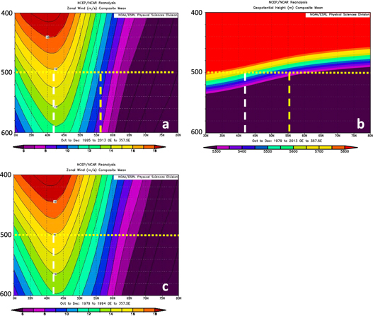
Figure 3. Zonal-mean zonal winds for fall (OND) from 1995 to 2013 (a) and from 1979 to 1995 (c). Corresponding zonal-mean geopotential heights for 1979–2013 are shown in (b). Dotted horizontal lines highlight the 500 hPa level, white dashed vertical lines indicate the latitude of maximum mean zonal winds at 500 hPa, and yellow dashed lines are the latitude of the waviest 500 hPa contour, as identified in [15].
Download figure:
Standard image High-resolution imageMeridional circulation index (MCI)
A key outstanding question in the proposed linkage between AA and jet-stream behavior is whether weakened poleward thickness gradients are causing the upper-level flow to become wavier. One measure of flow waviness is the ratio of the meridional (North/South) wind component to the total wind speed. We propose a simple metric to assess this characteristic of the flow: the MCI:

where u and v are the zonal and meridional components of the wind. When MCI = 0, the wind is purely zonal, and when MCI = 1 (−1), the flow is from the South (North). We note that a more meridional flow can result from either a stronger v and/or weaker u wind component through simple vector geometry. Whatever the cause, an increase in |MCI| indicates a wind vector aligned more North–South and reflects a changed flow direction. The speed of the meridional (v) wind may not change, as it is associated with East–West temperature gradients, but if the total wind vector becomes more meridional, then the flow is by definition 'wavier'. For example, a Northwesterly wind could shift to a North–Northwesterly wind solely through a reduction of the Westerly wind component. For this analysis, MCI is calculated from daily 500 hPa wind components between 20°N and 80°N at each gridpoint in NCEP Reanalysis fields.
Coincident anomalies in thickness, zonal winds, and MCI
In an effort to assess the effects of AA on waviness of upper-level winds, we compare coincident seasonal anomalies during the AA era relative to the period from 1981–2010. Anomalies in the 1000–500 hPa thicknesses are presented in the top panels of figures 4–7. During fall (OND, figure 7(a)), when sea-ice loss exerts its largest direct impact, the pattern of AA extends across much of the Central Arctic, while during spring (AMJ, figure 5(a)) and summer (JAS, figure 6(a)) the areas of positive thickness differences occur primarily over high-latitude land, likely in response to earlier snow melt [5]. In all seasons, positive thickness differences are evident in the Northwest Atlantic. This substantial regional and seasonal variability illustrates the challenge in detecting robust hemispheric-mean atmospheric responses to AA, resulting in the low statistical significance reported in some previous studies [15, 16, 28].
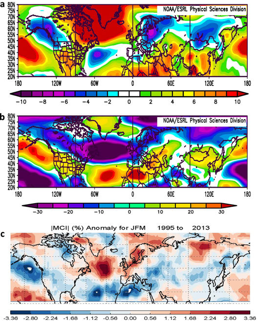
Figure 4. Anomalies in winter (JFM) (a) 1000–500 hPa thickness (m), (b) zonal wind at 500 hPa (m s−1), and (c) the absolute value of the MCI during 1995–2013 relative to 1981–2010. Data were obtained from NOAA/ESRL at http://www.esrl.noaa.gov/psd/.
Download figure:
Standard image High-resolution image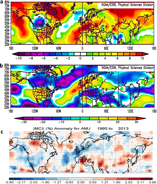
Figure 5. Same as figure 4 but for spring (AMJ).
Download figure:
Standard image High-resolution image
Figure 6. Same as figure 4 but for summer (JAS).
Download figure:
Standard image High-resolution image
Figure 7. Same as figure 4 but for fall (OND).
Download figure:
Standard image High-resolution imageThe middle panels of figures 4–7 present anomalies in zonal wind speeds at 500 hPa corresponding to anomalies in the poleward gradient of 1000–500 hPa thicknesses (top panels). Anomalies in |MCI| are shown in the bottom panels. Immediately obvious is the close association between the spatial patterns of weakened poleward gradients (regions where positive anomalies occur Northward of weaker or negative anomalies) and areas where zonal winds are weaker.
During winter and autumn (figures 4 and 7) a broad area of substantially weakened poleward gradient is evident across much of the Northern hemisphere mid-latitudes, particularly in the N. Atlantic and Northern Eurasia. These areas are closely matched by the spatial pattern of slower zonal winds, as would be expected according to the thermal wind relationship. Widespread positive anomalies in |MCI| also correspond to these regions. Changes in the meridional wind speed, however, are not correlated with either the changes in poleward gradient or zonal winds, suggesting that changes in |MCI| arise mostly because of changes in the zonal wind speed. These findings support the hypothesis that AA causes a more meridional character to the upper-level wind flow, but this change is achieved primarily via a reduction in Westerly winds rather than through an increase in meridional wind speeds.
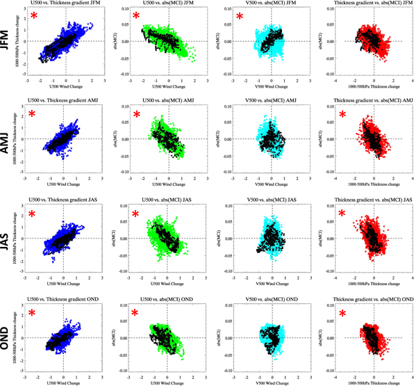
Relationships between these variables on a gridpoint-by-gridpoint basis are illustrated in scatterplots (figure 8). Gridpoints with weaker (stronger) poleward gradients tend to have larger (smaller) |MCI| values (red scatter-plots), particularly for gridpoints with the strongest (top decile) total winds, indicative of the jet stream. In all seasons, robust relationships between anomalies in the poleward gradient, zonal winds, and |MCI| are evident. Moreover, in spring, summer, and fall, the anomaly in 500 hPa zonal winds accounts for a much larger fraction of the variance in |MCI| than does the anomaly in the meridional wind component (variance explained by U500 in JFM, AMJ, JAS, OND = 0.42, 0.33, 0.61, 0.38; by V500 = 0.59, 0.02, 0.07, 0.001), suggesting that weakened zonal winds due to AA are the main factor driving the more meridional flow in these seasons. We also note that correlations between differences in 500 hPa meridional wind speeds with either the differences in poleward thickness gradient or zonal wind speed were small and insignificant, suggesting that changes in the |MCI| arise primarily because of changes in zonal wind speeds.
Figure 8. Seasonal scatterplots relating individual gridpoint values of anomalies during 1995–2013 for zonal and meridional winds at 500 hPa (U500, V500; m s−1), poleward gradients in 1000–500 hPa thickness (m deg−1), and |MCI| (unitless). Black asterisks indicate gridpoints corresponding to the highest 10% of total wind speed during 1995–2013 at 500 hPa, a proxy for the jet stream. Red asterisks indicate correlations between black points that exceed 50% and p ≪ .001.
Download figure:
Standard image High-resolution image
Extreme wave frequency
One aspect of the proposed linkage [1] that heretofore has been difficult to assess is whether the amplitude of planetary waves is increasing in response to strengthening AA. An alternative metric that we pursue here is the frequency of highly amplified jet-stream configurations. Single contours of daily mean 500 hPa height fields are used to identify 'extreme waves' in the jet stream. Representative contours (5600 m ± 50 m, except 5700 m ± 50 m in JAS) are selected to represent the streamline of the strongest 500 hPa winds as discussed previously, and we note that the selected contours shift little in latitude with time (figure 3). Data are analyzed in various longitude zones to identify days in which the difference between the maximum and minimum latitudes (ridges and troughs) of the contour within a region exceeds 35° of latitude. The threshold of 35° was selected to achieve a frequency of approximately 20 days per season (∼20%). Note that individual high-amplitude events, such as blocks and cut-off lows, often persist for several days, thus the frequency of events < frequency of high-amplitude days.
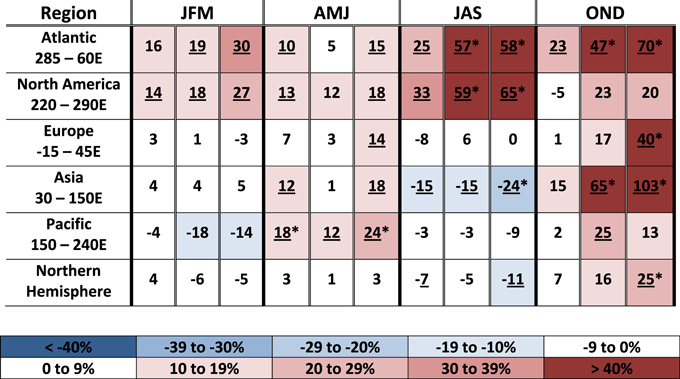
The frequency of occurrence of high-amplitude days is assessed in each season and for the AA era (1995–2013) relative to the pre-AA period (1979–1994). We repeat the analysis using two additional definitions of the AA era—1990–2013 and 2000–2013—to determine the sensitivity of differences in high-amplitude days to the time period selected for the AA era. The mean differences in frequency between these periods for each season and in selected regions are presented in table 1. Changes in frequency are expressed as a percentage relative to the pre-AA period. We also assess the choice of comparative years by randomly selecting 100 sets of a number of years from the pre-AA period corresponding to the length of each AA era, then calculating the standard deviation of the extreme-wave frequency in each set. Changes in frequency from the pre-AA period to the AA era that exceed one (two) standard deviation(s) are indicated by an underscore (asterisk).
Table 1. Percentage change in seasonal frequency of high-amplitude days from the pre-AA period to the AA-era assessed using three different initial years to define the AA-era: 1990–2013 (left column under each seasonal heading), 1995–2013 (middle column), and 2000–2013 (right column). High-amplitude days are identified when the difference between the maximum and minimum latitude of the selected daily 500 hPa height contour within a specified region exceeds 35° latitude (see text for contour selections). Underlined values indicate changes that exceed one standard deviation of wave frequencies during the pre-AA period as determined from 100 sets of randomly selected groups of years of the same number as the corresponding AA era (i.e., 24, 19, and 14 years beginning in 1979). Underlined and asterisked values exceed two standard deviations.
|
The changes in frequency are predominantly positive, indicating more frequent occurrences of highly amplified jet-stream configurations in the AA era. Seasonal and regional variations are generally consistent with the spatial patterns of anomalies in poleward thickness gradients shown in figures 4–7, particularly the most robust positive trends in extreme waves over the Atlantic and North American regions. We find a statistically significant negative correlation (Spearman's correlation = −0.30, >90% confidence) between the seasonal, regional-mean change in thickness gradient and the change in extreme-wave frequency. The autumn particularly stands out in table 1, with increases in extreme waves in all of the categories representing the post-AA period (1995–2013 and 2000–2013), as would be expected because fall exhibits the largest and most regionally consistent signal of AA. The Atlantic and North American regions also stand out, with increased frequencies in all post-AA categories. Decreased frequencies during Asian summer are consistent with recent cooling in North-Central Asia (figure 6), which strengthens the poleward gradient, drives stronger zonal winds, and results in a decreased |MCI|. Overall, the pattern of frequency change is consistent with expectations of a more amplified jet stream in response to rapid Arctic warming. Amplified jet-stream patterns are associated with a variety of extreme weather events (i.e., persistent heat, cold, wet, and dry) [22], thus an increase in amplified patterns suggests that these types of extreme events will become more frequent in the future as AA continues to intensify in all seasons. These results may also provide a mechanism to explain observed associations between sea-ice loss and continental heat waves [23, 29], cold spells [24, 30, 31], heavy snowfall [2], and anomalous summer precipitation patterns in Europe [32].
Discussion and conclusions
The Arctic has warmed at approximately twice the rate of the Northern mid-latitudes since the 1990s owing to a variety of positive feedbacks that amplify greenhouse-gas-induced global warming. This disproportionate temperature rise is expected to influence the large-scale circulation, perhaps with far-reaching effects. The North/South temperature gradient is an important driver of the polar jet stream, thus as rapid Arctic warming continues, one anticipated effect is a slowing of upper-level zonal winds. It has been hypothesized that these weakened winds would cause the path of the jet stream to become more meandering, leading to slower Eastward progression of ridges and troughs, which increases the likelihood of persistent weather patterns and, consequently, extreme events [1]. While weaker zonal winds have been observed in response to reduced poleward temperature gradients, the link to a wavier upper-level flow has not yet been confirmed [31, 33], although recent studies provide strong support of a mechanism linking sea-ice loss in the Barents/Kara Sea with amplified patterns over Eurasia during winter [24, 34] and summer [23]. We also note that the annual-mean NOAA-tabulated climate extreme index for the US [35] has increased by approximately one-third in the AA era relative to pre-AA years, though it is presently unknown whether rapid Arctic warming is a contributing factor.
Here we provide evidence demonstrating that in areas and seasons in which poleward gradients have weakened in response to AA, the upper-level flow has become more meridional, or wavier. Moreover, the frequency of days with high-amplitude jet-stream configurations has increased during recent years. These high-amplitude patterns are known to produce persistent weather patterns that can lead to extreme weather events [22, 23]. Notable examples of these types of events include cold, snowy winters in Eastern North America during winters of 2009/10, 2010/11, and 2013/14; record-breaking snowfalls in Japan and SE Alaska during winter 2011/12; and Middle-East floods in winter 2012/2013, to name only a few.
We assess anomalies in the poleward 1000–500 hPa thickness gradient during the AA era (since the mid-1990s) relative to climatology (1981–2010), along with corresponding changes in the zonal winds at 500 hPa and the waviness of the 500 hPa flow (|MCI|). While these time periods are short and certainly include effects of other natural fluctuations in the climate system, the conspicuous emergence of AA since the mid-1990s dictates this focused temporal analysis to identify responses of the large-scale circulation to this 'new' forcing. Future work will analyze climate model projections of a future with greater global warming and intensified AA. A recent study [36] documents a reduction in the frequency of atmospheric fronts under strong greenhouse forcing, particularly in high latitudes where the meridional temperature gradient relaxes the most, suggestive of more persistent weather patterns.
We find that in all seasons, the regions in which the poleward gradient weakens also exhibit weaker zonal winds (as expected via the thermal wind relationship) and consequently a more meridional, or wavier, flow character. This localized response is corroborated by seasonally varying, regional-scale increases in the frequency of amplified jet-stream configurations. The strongest response occurs during fall, when sea-ice loss and increased atmospheric water vapor augment Arctic warming, and a robust response is also evident during summer over North America and the Atlantic sectors, when the observed rapid decline of early-summer snow cover and the lower heat capacity of land promote a drying and warming of high-latitude land areas. Significant increases are observed in winter and spring, as well. These results reinforce the hypothesis that a rapidly warming Arctic promotes amplified jet-stream trajectories, which are known to favor persistent weather patterns and a higher likelihood of extreme weather events. Based on these results, we conclude that further strengthening and expansion of AA in all seasons, as a result of unabated increases in greenhouse gas emissions, will contribute to an increasingly wavy character in the upper-level winds, and consequently, an increase in extreme weather events that arise from prolonged atmospheric conditions.
Acknowledgments
The authors are grateful for funding provided by the National Science Foundation's Arctic System Science Program (NSF/ARCSS 1304097), to programming assistance from R Kyle Zahn, and for helpful suggestions from Dr John Walsh and two anonymous reviewers.