


Abstract
Cookstove use is globally one of the largest unregulated anthropogenic sources of primary carbonaceous aerosol. While reducing cookstove emissions through national-scale mitigation efforts has clear benefits for improving indoor and ambient air quality, and significant climate benefits from reduced green-house gas emissions, climate impacts associated with reductions to co-emitted black (BC) and organic carbonaceous aerosol are not well characterized. Here we attribute direct, indirect, semi-direct, and snow/ice albedo radiative forcing (RF) and associated global surface temperature changes to national-scale carbonaceous aerosol cookstove emissions. These results are made possible through the use of adjoint sensitivity modeling to relate direct RF and BC deposition to emissions. Semi- and indirect effects are included via global scaling factors, and bounds on these estimates are drawn from current literature ranges for aerosol RF along with a range of solid fuel emissions characterizations. Absolute regional temperature potentials are used to estimate global surface temperature changes. Bounds are placed on these estimates, drawing from current literature ranges for aerosol RF along with a range of solid fuel emissions characterizations. We estimate a range of 0.16 K warming to 0.28 K cooling with a central estimate of 0.06 K cooling from the removal of cookstove aerosol emissions. At the national emissions scale, countries' impacts on global climate range from net warming (e.g., Mexico and Brazil) to net cooling, although the range of estimated impacts for all countries span zero given uncertainties in RF estimates and fuel characterization. We identify similarities and differences in the sets of countries with the highest emissions and largest cookstove temperature impacts (China, India, Nigeria, Pakistan, Bangladesh and Nepal), those with the largest temperature impact per carbon emitted (Kazakhstan, Estonia, and Mongolia), and those that would provide the most efficient cooling from a switch to fuel with a lower BC emission factor (Kazakhstan, Estonia, and Latvia). The results presented here thus provide valuable information for climate impact assessments across a wide range of cookstove initiatives.

Content from this work may be used under the terms of the Creative Commons Attribution 3.0 licence. Any further distribution of this work must maintain attribution to the author(s) and the title of the work, journal citation and DOI.
1. Introduction
Cookstoves and residential sources account for approximately 20% of current black carbonaceous (BC) aerosol emissions (Bond et al 2007, Lamarque et al 2010). Policies targeting reductions to BC aerosol from cookstoves have garnered attention owing to their potential impacts on both climate and human health (e.g., Venkataraman et al 2010, Grieshop et al 2011, Department of State 2012, Anenberg et al 2013). Exposure to indoor and ambient fine particulate matter (PM) is responsible for approximately 4.3 and 3.2–3.7 million premature deaths per year, respectively (Anenberg et al 2010, Lim et al 2012), with solid fuel use contributing to approximately 0.5 million of the latter (Anenberg et al 2013). The total pre-industrial to present day effective radiative forcing (RF) of BC from all anthropogenic sources is 1.1 Wm−2 with a range of 0.17–2.1 Wm−2, which is similar in magnitude to the RF of prominent greenhouse gases (Ramanathan and Carmichael 2008, Bond et al 2013, Myhre et al 2013). This forcing is a combination of direct, semi-direct, and indirect effects that are in turn a function of chemical and physical processes in the atmosphere. The fraction of this forcing from cookstove BC emissions can not be directly attributed according to the cookstove fraction of global BC emissions owing the regional dependence of BC radiative forcing (RF) (Henze et al 2012).

Several uncertainties surrounding the net climate impacts of carbonaceous cookstove emissions complicate how mitigation efforts should be accounted for in environmental assessments (Grieshop et al 2009, Simon et al 2012, Lee et al 2013). Evaluating the climate impacts of actual BC cookstove emission reduction strategies requires accounting for species co-emitted with BC (particularly organic carbon (OC)), the chemical and physical processes affecting these species in the atmosphere, their climate impacts via multiple mechanisms, and the range of uncertainties associated with each of these components (Bond et al 2013, Myhre et al 2013). Previous studies have estimated a range of impacts from carbonaceous aerosol cookstove emissions (MacCarty et al 2008, Grieshop et al 2011, Freeman and Zerriffi 2014) based on the effects of co-emitted aerosol and gaseous precursor species that either have additional warming effects or counteract the effects of BC by reflecting incoming solar radiation. These co-emitted species depend on locally available fuels combined with traditional stoves and cooking methods (e.g., Bonjour et al 2013). A key consideration is the ratio of BC to total carbon emissions, referred to here as Φ. Variations in Φ can also be caused by differences in fuels, stove types, cooking methods and habitation, all of which vary regionally (Bond et al 2007, Jetter and Kariher 2009, Jetter et al 2012). In addition to carbonaceous aerosol emissions, other species co-emitted from residential cookstove use include trace amounts of aerosol precursors SO2 and NOx along with greenhouse gases CO, CH4, CO2, and, to a lesser extent, N2O (Smith et al 2000, Bhattacharya et al 2002, Roden et al 2006, Jetter et al 2012).
In addition to uncertainties related to both the total emissions and characterization of emissions for sectors which emit BC, difficulties in determining the net climate impacts from BC sources arise from the spatial relationships between these emissions and their impact on climate, which is more important for aerosols than for long lived, well-mixed greenhouse gases (Shindell and Faluvegi 2009, Henze et al 2012). BC emitted into regions with a low surface albedo have a smaller direct RF than BC emitted into regions with a high surface albedo (e.g., Ramanathan and Carmichael 2008, Henze et al 2012). Another factor that affects the climate impacts of carbonaceous aerosols is their atmospheric lifetime. This is a function of deposition loss rates, which are in turn a function of particle aging from hydrophobic to hydrophilic properties and local meteorology (Cooke et al 1999, Liu et al., 2001, Henze et al 2012, Shen et al 2014). There are also uncertainties in the absorption of BC particles owing to uncertainties in physical properties and aerosol mixing states (e.g., Jacobson 2001, Bond et al 2004, Lu et al 2015).
Recent work has explored the global impact of these types of uncertainties (emissions, aerosol properties, etc) and found the net global temperature impacts of aerosols from all biofuels to be rather ambiguous (Kodros et al 2015). Past studies have quantified the RF and climate impact of individual anthropogenic sectors through modeling studies which perturb the emissions from a specific species or sector, either globally or from a specific region (Fuglestvedt et al 2008, Unger et al 2010, Bauer and Menon 2012, Lund et al 2014). Other studies have provided more detailed analysis of RF specifically from global sources of carbonaceous aerosols (Koch and Del Genio 2010, Chung et al 2012). While all of these studies take into account aerosol indirect effects in some form, estimates of aerosol indirect RF for cookstoves, or carbonaceous aerosol in general, are highly variable (Pierce et al 2007, Chen et al 2010, Spracklen et al 2011, Kodros et al 2015). Further, strategies for mitigating cookstove emissions typically depend on local government and cultural factors, highlighting the need for analysis of the climate impacts of cookstove emissions at the national scale.
In this study, we expand on past work by evaluating temperature impacts of carbonaceous aerosol emissions from cookstove use in each country, taking into account co-emitted BC and OC, their emissions ratio as a function of fuel type, the spatial heterogeneity of direct RF, and the range of temperature responses likely owing to indirect forcing mechanisms. The previously mentioned studies used multiple forward model perturbations for their analysis. In contrast, here we use adjoint modeling to estimate the climate impacts of cookstove emissions simultaneously for all countries. Following Henze et al (2012), the GEOS-Chem adjoint model is used to estimate changes in direct RF with respect to carbonaceous aerosol emissions. Here we expand upon this approach to consider multi-model mean estimates and ranges for direct and indirect forcing from Boucher et al (2013) and Myhre et al (2013). Aerosol RF has strong spatial heterogeneity, and climate sensitivities to RF at different latitudes vary by up to an order of magnitude. To account for this, we estimate climate responses using absolute regional temperature potentials (ARTP) for regional surface temperature over land parameterized from a chemistry-climate model (Shindell and Faluvegi 2009, Shindell 2012). This allows us to estimate temperature responses to RF within different latitude bands. We also bound the total magnitude of the temperature response from removal of cookstove emissions, changes in cookstove efficiencies, and changes in Φ for each country.
2. Methods
2.1. GEOS-Chem forward and adjoint modeling
Here we provide a brief overview of the models and methodology used for this paper, which are explained in detail in the Supporting Information. Results were generated using the global GEOS-Chem chemical transport model and its adjoint based on year 2000 historical emissions from Lamarque et al (2010). Grid-scale adjoint sensitivities were then multiplied by a grid-scale cookstove emissions inventory constructed from the biofuel emissions inventory from Bond et al (2007) and the country-level percent solid fuel use from Bonjour et al (2013), as described in Supporting Information, yielding estimates of the biofuel emissions from the fraction of the population of each country that use solid fuels for cooking with an additional regional correction factor to account for non-cookstove carbonaceous aerosol emissions. This adjoint approach allows us to calculate (at the cost of 12 forward model calculations) grid-cell contributions to changes in the regional direct RF due to solid fuel cookstove use that would have otherwise required ∼105 forward model simulations.

2.2. Direct, indirect and semi-direct RF estimates
Several intermodel comparisons have shown a wide range of estimates for aerosol direct and indirect effects owing to various parameterizations regarding the chemical and physical properties of carbonaceous aerosol and their interaction with the environment (UNEP and WMO 2011, Boucher et al 2013, Myhre et al 2013, Bond et al 2013). To account for this range, following an approach used in the UNEP Integrated Assessment Report, we rescale the calculated direct RF to match the species-specific estimated RF from Myhre et al (2013), shown in table 1. We also apply additional scaling factors to account for indirect and semi-direct effects, assuming that their magnitudes scale proportionally with direct RF (Boucher et al 2013). This simple relationship may not hold on smaller regional scales, where variations in aerosol and cloud microphysics may dominate. However, globally many chemistry-climate models exhibit a relationship between direct and indirect effects that falls within the range encompassed by the scaling factors applied here (e.g., Shindell et al 2013). In addition, we use the adjoint model to calculate the contribution of emissions in any grid cell to deposition of BC onto snow and sea ice. These sensitivities are used to spatially distribute the global estimated BC snow albedo effect of 0.15 Wm−2 (UNEP and WMO 2011, Bond et al 2013) on an emission per grid-cell basis, as shown in figure S.3.
Table 1. Scaling factors for direct radiative forcing () and various secondary radiative effects () for BC, OC and secondary inorganic aerosol (SIA).


| Type | Species | Lower | Central | Upper |
|---|---|---|---|---|
| BC | 1.840 | 2.761 | 3.681 | |
| OC | 0.695 | 1.595 | 2.394 | |
| SIA | 0.256 | 0.567 | 1.001 | |
| BC | −0.143 | 1.000 | 1.471 | |
| OC | 1.019 | 1.560 | 1.740 | |
| SIA | 1.446 | 2.214 | 2.470 |


These scaling factors and BC snow ice albedo sensitivities are combined for each grid cell, i, and species, k, for a given forcing region, τ (Arctic, NH mid-latitudes, Tropics and SH Extratropics), in equation (1),
where is the rescaled complete RF sensitivity, is the RF sensitivity calculated by the GEOS-Chem adjoint model and is the yearly averaged RF sensitivity from the BC snow/ice albedo change.


2.3. Temperature response estimates
Temperature responses are estimated from the application of ARTP coefficients to regional RF sensitivities in four different latitude bands calculated with the adjoint model. These ARTP coefficients are developed following the approach of Shine et al (2005) for global temperature potentials, extended in Shindell and Faluvegi (2010) and Shindell (2012) to regional potentials. These are based on regional climate sensitivities derived from the transient chemistry-climate-ocean GISS model simulations of Shindell and Faluvegi (2009) and account for both ocean inertia and the influence of local and remote aerosol direct and indirect forcings. These ARTP coefficients represent the magnification of regional sensitivities relative to the global mean equilibrium climate sensitivity of 1.06 C per W m−2 (corresponding to 3.9 C response for a doubling of CO2). Temperature responses estimated using the ARTP coefficients have been shown (Shindell 2012) to estimate regional climate responses within 20% (at 66–95% confidence intervals) of the response calculated using three independent full chemistry-climate models; the uncertainty is less when considering the global climate response as a combination of area-weighted regional responses. To evaluate the impact of using this method to capture spatially heterogeneous forcings and responses, the temperature response to emissions perturbations is calculated in two different ways. The first method is to calculate the change in global RF for a specific species k (BC and OC in this case) and each grid cell i and multiply it by the global mean sensitivity (GMS) as shown in equation (2),

where is the emissions perturbation and is the rescaled global RF sensitivity calculated using the adjoint model as shown in equation (1). The second method is to calculate the temperature response in a region, γ, using absolute regional temperature potential coefficients (ARTP) (Shindell and Faluvegi 2009, Shindell 2012). This method estimates the steady state temperature response from changes in regional RF (forcing regions τ defined in section A.3) based on the following equation:


is the steady state temperature response in each region, which can then be converted to a global averaged temperature change using the area ratio of each response region


The contribution of an emission in an individual grid cell to the overall temperature change is thus
3. Results
3.1. Regional versus global climate response
We first evaluate the consequences of using regional rather than global temperature response coefficients. For species where the RF does not have a strong dependence on latitude, such as OC, the estimated global average temperature response is similar using both methods. For example, the predicted temperature response due to removal of biofuel OC emissions everywhere is 0.10 K using the global method (equation (2)) and 0.11 K using the ARTP method (equation (4)). In contrast, the removal of BC biofuel emissions yields a global average temperature change of −0.13 K using the global method and −0.22 K using the ARTP method. Figure 1 shows each grid cell's contribution to global surface temperature change calculated using the global versus ARTP method, colored by each ARTP response region (γ). The magnitudes are similar for most points in the Tropics, as the climate response in the Tropics follows the global surface temperature response (Shindell and Faluvegi 2009). The largest deviations from the 1:1 line are due to larger ARTP predicted temperature responses in the Arctic and Northern Hemisphere mid-latitudes and smaller ARTP predicted temperature response in the Southern Hemisphere combined with differences in the calculations of for different regions compared to This means that in most regions the ARTP method predicts a larger contribution to the global temperature perturbation than the globally averaged temperature perturbation owing to the higher climate sensitivities as well as higher RF efficiencies for BC in northern latitudes. These differences in temperature response highlight the value of using the ARTP method for short-lived species that have latitudinally variable RF sensitivities. Therefore, the rest of this paper will present temperature changes using the ARTP method (equation (4)).


Figure 1. Comparison between contributions of 2.5° grid-cell removal of biofuel emissions to the global mean surface temperature using the ARTP method (x-axis) and the Global Method (y-axis) for (a) BC and (b) OC. Colors represent the location of the grid cells for the emissions inventory.

Download figure:
Standard image High-resolution image3.2. Temperature response from cookstove emissions
This section explores how uncertainties in emissions, emission characterizations, and RF mechanisms contribute to temperature change estimates from cookstove emissions reductions. By using the emissions from cookstoves as calculated with equation (S.1), the central estimate for the total temperature change due to removal of all carbonaceous aerosol emissions from residential cookstoves is a cooling of 0.06 K (0.06 K warming from removal of OC and 0.12 K cooling from removal of BC).
Analysis of the BC and OC emission factors shown in figure S.1 creates a range of Φ of 0.24 +/− 0.09 corresponding to the mean and standard deviation of all emissions factors. We combine this with the upper and lower estimates for RF scaling factors (table 1) to estimate bounds for the global surface temperature change due to cookstove emissions. Figure 2 plots the ranges in surface temperature response to removal of cookstove emissions for a range of uncertainties in the RF from carbonaceous aerosols (table 1) and the value of Φ for cookstove emissions.
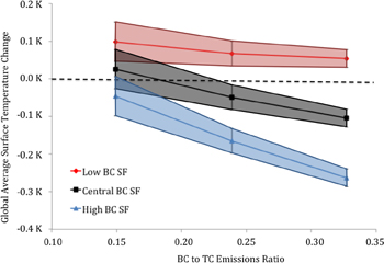
Figure 2. Bounds for the global temperature response due to removal of cookstove emissions (y-axis) for a given Φ (x-axis). Lines correspond to the central, high, and low BC radiative forcing scaling factors shown in table 1, and the ranges for each line correspond to the central, high, and low OC radiative forcing scaling factors.
Download figure:
Standard image High-resolution imageFigure 2 shows a large range of uncertainty in the overall temperature impacts due to remove of cookstove emissions based on the effective RF efficiency of BC and OC along with the characterization of the BC to total carbon emissions ratio for solid fuel use. This plot shows that for low Φ, 0.15, the effects from OC emissions dominate, leading to a central estimate of a net warming of 0.03 K along with higher uncertainties due to the current understanding of OC RF. The opposite is true for high Φ, 0.33, for which BC dominates the temperature impacts and the potential temperature change due to removal of cookstove emissions is a cooling of as much as 0.28 K. In order to further understand the global climate impacts of cookstove use, the assumptions regarding solid fuel use are further explored below by considering individual national-scale contributions to the overall temperature change.
We next consider the climate impacts of cookstove emissions from each country in which greater than five percent of the population uses solid fuels. Using equation (5), we calculate the contribution of cookstove aerosol emissions in each grid cell to global surface temperature change. These results are then aggregated by country. Figure 3 shows the top 15 countries in terms of the magnitude of the cooling resulting from removal of cookstove removal aerosol emissions, where the temperature change has been separated into species-specific direct and indirect effects. In addition to countries with the largest cooling impact, Brazil and Mexico have been included to show the contrast between countries with cookstove aerosol cooling effects and countries with the largest cookstove aerosol warming effects. The error bars show the range of estimates obtained using the different assumptions regarding RF scaling factors (shown in table 1) and assumptions for country specific values for Φ. Note that for BC, the semi and indirect effects only contribute to the range but do not perturb the central estimate. In general, the range of estimates in the temperature impact tends to be a function of emissions, where countries with larger emissions mostly have larger uncertainties. Second, the centering of the range of estimates around the central value is a function of Φ. Countries with a Φ around 0.15 (e.g., Ukraine and Kazakhstan, see figure S.6) will have ranges that are skewed toward a stronger cooling than countries with a Φ greater than 0.2 (e.g., India and China) where the ranges are relatively centered. This is not purely a function of Φ though, as each country's mean RF sensitivity with respect to BC and OC also plays a role in the range and centering of the ranges. Finally, this plot shows the snow deposition albedo effect and its relative importance for each country; Nepal has an approximately equal impact via the snow-albedo effect as the direct BC effect, while Nigeria has a near-zero snow-albedo effect.

Figure 3. Each country's contribution to global surface temperature change broken down into the individual components. The uncertainty ranges are taken from assumptions about the radiative effects shown in table 1 and the reasonable range of Φ shown in figure 2. BC semi-direct and indirect effects perturb only the upper and lower bounds, not the central estimate. China and India are shown on the scale on the left, and all other countries use the scale on the right.
Download figure:
Standard image High-resolution imageWe next consider how individual countries rank in terms of several metrics, using the central estimate for each country in each case. Table 2 shows each of the different rankings, which are defined and explained below. We first consider each country's contribution to overall temperature change due to removal of cookstove aerosol emissions (see figure 4(a)) in column two of table 2. With the exception of China, India and Nigeria, the ranking of countries with the largest contribution to total temperature change is not the same as the ranking of countries with the largest emissions (first column of table 2); instead, the temperature change is a function of the sensitivity of temperature with respect to emissions of BC and OC and the characterization of Φ within that country.

Figure 4. Country-level contributions to global temperature change using various metrics: (a) globally averaged surface temperature change from removal of cookstove emissions including direct, semi-direct and indirect effects (total temperature change for India = −6.2 mK and China = −33.1 mK) calculated using equation (4), (b) cookstove mitigation efficiency, i.e., the total temperature effect from removal of cookstove emissions per total cookstove emissions, (c) temperature effect per total biofuel emissions corresponding to a 10% reduction in Φ from cookstove use. Kazakhstan (−86.5), Estonia (−78.9), and Latvia (−62.0) are outside of the scale shown in panel (c). Countries in grey have less than 5% total population using solid fuels for cooking.
Download figure:
Standard image High-resolution imageTable 2. Rankings of contribution to total temperature change and emissions metrics from the largest annual emissions (column 1), cooling impact from removal of annual cookstove emissions (column 2), or efficiency in terms of cooling effect per emission (columns 3 and 4).
| Rank | Carbonaceous aerosol emissions (Gg C) | Global temperature change contribution (mK) | Cookstove change efficiency (mK(kg C)−1) | Fuel switching efficiency (mK(kg C)−1) |
|---|---|---|---|---|
| 1 | China | China | Kazakhstan | Kazakhstan |
| 2 | India | India | Estonia | Estonia |
| 3 | Ethiopia | Uzbekistan | Mongolia | Latvia |
| 4 | Bangladesh | Ukraine | Latvia | Lithuania |
| 5 | Congo, DRC | Nigeria | Uzbekistan | Ukraine |
| 6 | Nigeria | Kazakhstan | Lithuania | Mongolia |
| 7 | Kenya | Kyrgyzstan | Kyrgyzstan | Uzbekistan |
| 8 | Indonesia | Tajikistan | Georgia | Kyrgyzstan |
| 9 | Tanzania | Azerbaijan | Ukraine | Georgia |
| 10 | Vietnam | Pakistan | Armenia | Armenia |
We next consider the results ranked according to the countries that are most efficient in terms of temperature change for a given reduction of emissions. Figure 4(b) shows countries colored by their contribution to temperature change per total carbonaceous aerosol emission, and column three of table 2 shows the highest ranked countries according to this efficiency metric. Since many high performance stoves offer a significant reduction in the total carbonaceous aerosol emission factors per fuel used (Jetter et al 2012), the policy implication of this metric is to show in which countries implementing new stove technologies will result in the largest global cooling per emission reduced. These results also highlight countries where estimates of the total temperature impact (figure 4(a)) are most sensitive to uncertainties in cookstove emission inventories. The countries that rank high in terms of efficiency (blue) differ from countries ranked high in figure 4(a). Since the former have a larger absorptive effect from BC than reflective effect from OC, each stove replaced will have a greater climate impact. Conversely, it is inefficient to implement new stoves in countries that rank very low in this metric (red) and in some cases may even result in a net warming through removal of reflective OC.
Another metric which gives important information beyond the total contribution to temperature change is based on characterization of the fuels in a country, i.e., Φ (shown in figure 4(c) and the fourth column of table 2). This metric first calculates the increased cooling effect due to a −0.10 perturbation of Φ owing to a change of fuel type to one with a lower BC to OC ratio, which is optimal for reducing the warming effects of emissions due to biofuel use. This temperature change can then be turned into an efficiency metric by dividing by the total carbonaceous emissions in a country. This metric then gives the temperature response per kilogram of fuel changed for each country. An added benefit of this metric is that it highlights countries that are least robust in terms of estimating temperature impacts owing to uncertainties in Φ.
4. Discussion and conclusions
Using the GEOS-Chem adjoint model we have estimated the temperature impacts per amount of carbonaceous aerosol cookstove emissions on a 2.5° scale. These estimates include parameterizations for indirect and semi-direct aerosol RF and the contribution of regional RF to steady-state climate response. Accounting for spatially heterogeneous RF and climate sensitivities across four zonal bands in our approach is found to double the estimated cooling owing to removal of BC emissions compared to estimates based on global forcing and climate sensitivities. We find the total aerosol climate effect from removal of cookstove emissions (estimated here as the emissions from solid biofuel use from populations that use solid fuel for cooking) ranges from a potential warming of 0.16 K to a cooling of −0.28 K when evaluated for published ranges for both the RF effects and characterization of the BC to total carbon emission factor. We also develop and apply a new adjoint based method for attributing the global RF of albedo feedback from deposition of BC onto snow and sea ice due to emissions from individual countries. We find this effect is approximately the same order of magnitude as the direct effect for emissions from Nepal and other high altitude mountainous countries.

By examining the climate impacts of country-specific cookstove emissions, several trends are evident that have importance for policy decisions regarding cookstove interventions and implementation. China and India by far have both the largest carbonaceous cookstove emissions as well as the largest temperature change for national removal of these emissions, which is very likely a net cooling given the current range of estimated forcing magnitudes and emissions factors. In contrast, Nigeria and other countries in Africa with large cookstove emissions have cooling effects that are less certain.
Kazakhstan, Estonia and Mongolia are the most efficient countries for impacting global temperatures by implementing cookstoves, and emissions reductions in former republics of the USSR (e.g., Uzbekistan, Kyrgyzstan, etc) have the smallest likelihood of warming, relative to the magnitude of their central estimate for cooling. In general, cookstove emissions at higher latitudes have larger climate impacts per kg BC emitted due to RF and climate sensitivities that are both relatively large in those regions, which results in a difference between BC and OC contributions to climate impact that is greater than one order of magnitude. In contrast, for countries in Central and South America such as Dominica, Brazil, Mexico, and El Salvador, the climate response to cookstove emission reductions is relatively inefficient and may even lead to a net warming due to the larger impacts of OC emissions. This does not mean that cookstove interventions in such countries are not warranted from a climate perspective, as they may have a large climate impact based on co-emitted greenhouse gases or may be potential targets for improved thermal efficiency or fuel switching.
Through the use of scaling factors, the results presented here consider a range of climate impacts due to carbonaceous aerosol emissions from cookstoves owing to uncertainties in RF and emissions properties. The models used in Myhre et al (2013) and Boucher et al (2013) represent a range of parameterizations for various chemical and physical properties including, but not limited to, aerosol mixing state, BC aging, aerosol-cloud interactions, and optical properties; although several additional sources of uncertainty warrant consideration for future work. First, there is uncertainty in the cookstove emissions inventory itself, which may be biased for reasons discussed in detail in section A.2. These biases would impact our estimate of absolute temperature impacts from removal of cookstove carbonaceous emissions, although they would not affect our estimates of the efficiency of carbonaceous aerosols emissions reductions or fuel switching on climate (which are linear responses). We have also not considered countries with less than 5% of the population using solid fuel for cooking—thus some high latitude countries with large populations (i.e., Russia and Canada) may have large temperature impacts that have not been considered here—nor have we distinguished between cooking with modern woodstoves versus traditional open-air cookstoves.
In using the ARTP coefficients we are using a climate model parameterization. This parameterization is based off the GISS-ER model, although Shindell (2012) the calculated regional climate response is within 20% (at a 95% confidence interval) of the response calculated using a suite of full chemistry-climate models and the uncertainty is less than that when considering the global climate response as a combination of regional responses.
Another source of uncertainty arises from not rigorously treating secondary organic aerosols (SOAs) in this analysis owing to the nascent state of understanding of SOA sources and formation mechanisms. We can estimate an upper range of the impact of SOA relative to OC using speciation of biofuel non-methane volatile organic compounds (NMVOC) from Streets (2003) and NMVOC cookstove emissions factors from Grieshop et al (2011), which are approximately 2:1 relative to OC. Considering both aromatic compounds and other non-speciated compounds to be SOA precursors we estimate the total emissions of SOA precursors to be at most 38% (17% aromatics and 21% other) of total NMVOC emissions from cookstove use. For a 100% upper bound on SOA yield from these emissions, the climate impact from SOA is globally at most 76% of the OC impact. For the high northern latitude countries like Uzbekistan and Kazakhstan, OC impacts are negligible when compared to BC impacts, meaning that the inclusion of SOA would have a very small effect. In contrast, a net warming can not be ruled out for countries like Nigeria and Bangladesh, while the net effect in India and China would still likely be a cooling.
Lastly, with the exception of BC deposition albedo, we have treated aerosol indirect effects as being spatially uniformly proportional to direct effects. While this assumption is used in many models dealing with changes in the global mean impacts (UNEP and WMO 2011, Bond et al 2013, Boucher et al 2013), other studies have shown that the spatial distribution of these effects can be regionally heterogeneous (Pierce et al 2007, Bollasina et al 2011, Kodros et al 2015). Future work should explore these sources of uncertainty to further understand the net impacts of cookstove use and to provide improved information to policymakers, potentially further using adjoint sensitivity analysis to examine spatial heterogeneity in the relationship between aerosol indirect forcing and emissions locations (e.g., Karydis et al 2012, Moore et al 2013).
Acknowledgments
The research described in the article has been funded wholly or in part by the US Environmental Protection Agency's STAR program through grant 83521101, although it has not been subjected to any EPA review and therefore does not necessarily reflect the views of the Agency, and no official endorsement should be inferred. In addition this work is possible through NASA AQAST (NNH09ZDA001N) and support from the NASA HEC computing facilities.