


Abstract
The spatial context is critical when assessing present-day climate anomalies, attributing them to potential forcings and making statements regarding their frequency and severity in a long-term perspective. Recent international initiatives have expanded the number of high-quality proxy-records and developed new statistical reconstruction methods. These advances allow more rigorous regional past temperature reconstructions and, in turn, the possibility of evaluating climate models on policy-relevant, spatio-temporal scales. Here we provide a new proxy-based, annually-resolved, spatial reconstruction of the European summer (June–August) temperature fields back to 755 CE based on Bayesian hierarchical modelling (BHM), together with estimates of the European mean temperature variation since 138 BCE based on BHM and composite-plus-scaling (CPS). Our reconstructions compare well with independent instrumental and proxy-based temperature estimates, but suggest a larger amplitude in summer temperature variability than previously reported. Both CPS and BHM reconstructions indicate that the mean 20th century European summer temperature was not significantly different from some earlier centuries, including the 1st, 2nd, 8th and 10th centuries CE. The 1st century (in BHM also the 10th century) may even have been slightly warmer than the 20th century, but the difference is not statistically significant. Comparing each 50 yr period with the 1951–2000 period reveals a similar pattern. Recent summers, however, have been unusually warm in the context of the last two millennia and there are no 30 yr periods in either reconstruction that exceed the mean average European summer temperature of the last 3 decades (1986–2015 CE). A comparison with an ensemble of climate model simulations suggests that the reconstructed European summer temperature variability over the period 850–2000 CE reflects changes in both internal variability and external forcing on multi-decadal time-scales. For pan-European temperatures we find slightly better agreement between the reconstruction and the model simulations with high-end estimates for total solar irradiance. Temperature differences between the medieval period, the recent period and the Little Ice Age are larger in the reconstructions than the simulations. This may indicate inflated variability of the reconstructions, a lack of sensitivity and processes to changes in external forcing on the simulated European climate and/or an underestimation of internal variability on centennial and longer time scales.
Export citation and abstract BibTeX RIS

Original content from this work may be used under the terms of the Creative Commons Attribution 3.0 licence. Any further distribution of this work must maintain attribution to the author(s) and the title of the work, journal citation and DOI.
Introduction
Europe has experienced a pronounced summer (June–August) warming of approximately 1.3 °C over the 1986–2015 period (figure 1b), accompanied by an increase of severe heat waves (length, frequency and persistency), most notably in 2003, 2010 and 2015 (Luterbacher et al 2004, Schär et al 2004, Beniston 2004, 2015, Della-Marta et al 2007, García-Herrera et al 2010, Barriopedro et al 2011, Rahmstorf and Coumou 2011, IPCC 2012, Russo et al 2015). The likelihood of occurrence of heatwaves and extremely hot summers in Europe has risen significantly in the first part of the 21st century—a trend mainly attributed to anthropogenic forcing (Stott et al 2004, Christidis et al 2015). Initiatives to benchmark European summer warming and the occurrence of extreme events have been launched to improve our understanding of the climate system and thus reduce and quantify uncertainties in the magnitude of projected future climate change (Hegerl et al 2011, Christidis et al 2012, 2015, Goosse et al 2012a). Paleoclimatic data covering the past 2000 yr provide a crucial perspective for characterizing natural decadal to centennial time-scale changes and to put recent climate change into a long-term perspective. Paleoclimatological advances over the past decade include: (i) the production of new proxy records and new compilations on a regional basis (e.g. PAGES 2k Consortium 2013, 2014, Büntgen et al 2016, Schneider et al 2015); (ii) developments in multi-proxy reconstruction methodologies (e.g. Tingley and Huybers 2010a, 2010b, Smerdon 2012, Werner et al 2013, Neukom et al 2014, Guillot et al 2015, Werner and Tingley 2015); and (iii) development of comparison strategies between model experiments and reconstructions to assess the role of external forcing, feedbacks, and internal variability on the historical course of climate (e.g. Hegerl et al 2011, Bothe et al 2013a, 2013b, Fernández-Donado et al 2013, 2015, Schmidt et al 2014, Barboza et al 2014, Coats et al 2015, Moberg et al 2015, PAGES2k-PMIP3 Group 2015, Stoffel et al 2015, Tingley et al 2015). Additionally, new standards have been reached regarding the collection and archiving of proxy data (e.g. PAGES 2k Consortium 2013, 2014), estimation methods for past climate variability and associated uncertainties, and the analysis of uncertainties related to model forcing (Fernández-Donado et al 2013, 2015 and references therein). In a coordinated effort, the PAGES 2k Consortium (2013) presented a global dataset of proxy records and associated temperature reconstructions for seven continental-scale regions, including Europe and the Mediterranean region. Eleven annually resolved tree-ring width (TRW) and density records and documentary records from ten European locations were used in an ensemble composite-plus-scale (CPS) reconstruction of mean European summer land temperature for the past two millennia. Here we build upon these results and provide new estimates of European summer temperature variability over more than the past two millennia. We present: (i) annually-resolved gridded summer temperature fields over Europe for the period 755–2003 of the Common Era (CE) based upon Bayesian hierarchical modelling (BHM; Tingley and Huybers 2010a, 2010b, 2013, Werner et al 2013; see methods and supplementary online material, SOM, for details) integrating a number of recently developed millennium length tree-ring records and historical documentary proxy evidence including a comparison with independent long-instrumental and proxy based regional summer temperature reconstructions (see data section; SOM); (ii) two reconstructions of mean European (weighted average over European land areas, see data) summer temperatures back to 138 BCE based on the CPS method and the averaged ensemble BHM. The CPS based reconstruction is similar to the one published for Europe by the PAGES 2k Consortium (2013), although it employs a slightly different proxy set (see data and SOM); (iii) a comparison between our new reconstructions and an ensemble of millennium-length climate model experiments (Masson-Delmotte et al 2013) in order to assess consistency with changes in external forcing and the simulated climate variability over Europe; and (iv) spatial differences between simulated and reconstructed European summer temperature for the periods of the 'Medieval Climate Anomaly' (MCA, 900–1200 CE), the 'Little Ice Age' (LIA, 1250–1700 CE), and present-day (1950–2003 CE).
Data
Proxy and instrumental data
Nine annually resolved tree-ring width (TRW, Popa and Kern 2009, Büntgen et al 2011, 2012), maximum latewood density (MXD; Büntgen et al 2006, Gunnarson et al 2011, Esper et al 2012, 2014), combined MXD and TRW (Dorado Liñán et al 2012) and documentary historical records (Dobrovolný et al 2010) were used for the reconstructions (table S1). Their locations encompass the region from 41° to 68° N and from 1° to 25° E (figure 1(a); SOM). The reconstructions target the period 138 BCE to 2003 CE, the last year for which all proxies are available. Records were selected based upon their seasonal summer temperature signals, their record length (700+ years for tree-ring records), and sample replication. We excluded the PAGES 2k Consortium (2013) TRW records from Slovakia (Büntgen et al 2013) and Albania (Seim et al 2012) that were found to lack significant correlations with European summer temperature variability. Furthermore, the Torneträsk MXD record of Briffa et al (1992) that originally ends in 1980 CE, was substituted with the updated and newly processed data of Melvin et al (2013) and Esper et al (2014).
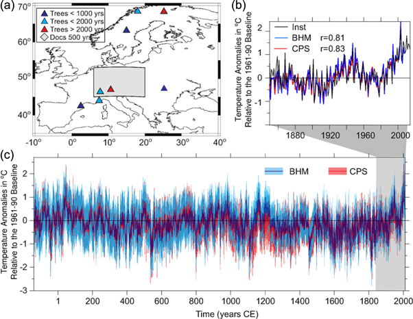
Figure 1. (a) Spatial distribution of proxy records used in the reconstructions. (b) Comparison of the instrumental mean summer temperature anomalies for Europe (1850–2015) with the mean BHM-based and CPS reconstruction anomalies 1850–2003. (c) CPS- and area-weighted mean BHM-based reconstructions of European summer temperature anomalies and 95% confidence intervals (shading in respective colour) over the period 138 BCE–2003 CE (all anomalies are with respect to the 1961–90 climatology).
Download figure:
Standard image High-resolution imageCalibration data for the European summer temperature reconstructions were derived from the CRUTEM4v data product, comprising monthly mean surface air temperature anomalies (with respect to 1961–1990CE) on a 5° × 5° land-only grid spanning the period 1850–2010 CE (Jones et al 2012). The region 35°–70° N/10° W–40° E was selected, excluding grid cells over Iceland and small North Atlantic islands. Thus, 61 grid cells were retained. Missing months in the selected cells were infilled using the regularised expectation maximisation algorithm with ridge regression (Schneider 2001) to yield a time-continuous monthly anomaly grid over the period 1850–2010 CE (see SOM for details). The resulting data were used to calculate mean June–August (JJA) temperatures of each year and each grid cell, from which an area-weighted (North et al 1982) mean summer temperature index was computed. For the BHM based reconstruction, the original, non-infilled data were used (see methods and SOM for details). A comparison between the seasonal mean temperatures for the European domain using the raw (non-infilled) data and the temporally and spatially continuous (infilled) field is presented in figure S1 (SOM). Correlation coefficients between the proxy data and both the European mean summer temperature and local JJA grid cell temperatures from the infilled dataset for the period 1850–2003 CE are given in table S2 (SOM).
Atmosphere-ocean general circulation model (AOGCM) data
The European summer temperature reconstructions are compared with fully coupled state-of-the art AOGCM simulations. The model-data comparison is based on 37 millennium-length simulations (see table S14) performed with 13 different AOGCMs. The ensemble includes eleven simulations from the Coupled Model Intercomparison Project Phase 5—Paleo Model Intercomparison Project Phase 3 (CMIP5/PMIP3; Braconnot et al 2012, Taylor et al 2012, Masson-Delmotte et al 2013) and 26 pre-PMIP3 additional simulations discussed in Fernández-Donado et al (2013). Aside from differences in model complexity and resolution, the most notable asset of the ensemble is the range of variation in applied external forcing configurations. The models consider different forcing factors and are also based on different forcing reconstructions. The CMIP5/PMIP3 simulations follow the forcing protocol outlined in Schmidt et al (2011, 2012), while the pre-PMIP3 simulations use a larger variety of forcing reconstructions (see Fernández-Donado et al 2013). The range in the applied external forcing configurations is largest for total solar irradiance (TSI). This relates most to the re-scaling and conversion of raw estimates (e.g. 10Be or 14C) into changes in incoming shortwave radiation in units of Wm−2 (Solanki et al 2004, Steinhilber et al 2012) rather than the character of the temporal evolution over the past 2000 yr. The re-scaled TSIs used for the climate simulations can be classified into two groups according to the magnitude of their low frequency variations, thus leading to two sub-ensembles of simulations (Fernández-Donado et al 2013): one involving stronger solar forcing variability (used in some pre-PMIP3 simulations) with a percentage of TSI change between the Late Maunder Minimum (LMM; 1675–1715 CE) and present >0.23%, denoted here SUNWIDE; another, with weaker solar forcing scaling (used by the CMIP5/PMIP3 experiments and some pre-PMIP runs) characterised by a TSI change between LMM and present <0.1%, denoted here SUNNARROW (see SOM for more details). On hemispheric scales, the highest estimates of solar forcing seems to yield a discrepancy between forced simulations and reconstructions (Schurer et al 2014). Regionally and seasonally the effect of solar forcing may be enhanced due to dynamic feedbacks that are largely missing in models (see Gray et al 2010).
Methods
European mean summer temperature reconstructions covering more than 2000 yr were created by using BHM and CPS. The two methods are based on different statistical assumptions regarding the proxy records and their associated temperature signals. Both methods provide uncertainty estimates and have been tested with synthetic data in pseudo-proxy experiments (Werner et al 2013, Schneider et al 2015). BHM was applied to derive spatial fields of summer temperature. We show the area-weighted mean back to 138 BCE, but limit the analysis of the spatial results to the period 755–2003 CE due to the low number of proxies before that period.
Composite-plus-scaling
A nested CPS (e.g. Jones et al 2009, PAGES 2k Consortium 2013, Schneider et al 2015) reconstruction was computed using eight nests reflecting the availability of predictors back in time (see table S1 for the initial year of each nest). A CPS reconstruction was computed for each nest by normalising and centring the available predictor series over the calibration interval (1850–2003 CE). A composite for each nest was then calculated by weighting each proxy series by its correlation with the European mean summer temperature. Finally, each composite was centred and scaled to have the same variance as the target index during the calibration period. CPS was implemented using a resampling scheme for validation and calibration (e.g. McShane and Wyner 2011, Schneider et al 2015) based on 104 yr for calibration and 50 yr for validation (the last year of the uniformly available predictor series is 2003, providing 154 yr of overlap with the target index, see SOM for details). Detailed validation statistics, with associated information across all reconstruction ensemble members within each nest, are provided in the SOM (tables S3 and S4). The limited number of proxies might be an important caveat for the reconstructions. Figure S3 shows the comparison of the eight nests in the CPS-based reconstructions of mean European summer temperature anomalies for the period 138 BCE–2003 CE. There are small differences between nests, but the covariance among each nest is remarkably consistent across all of the nests during their periods of overlap. The new CPS reconstruction, in the absence of the two predictors used by the PAGES 2k Consortium (2013) and employing the updated Torneträsk MXD record (Esper et al 2014), is virtually identical to the original PAGES 2k reconstruction over the full duration of the two reconstructions (Pearson's correlation coefficient of 0.99; figure S2).
Bayesian hierarchical modelling (BHM)
Bayesian inference from a localised hierarchical model (Tingley and Huybers 2010a, 2010b, 2013) was used to derive a gridded summer temperature reconstruction from 138 BCE to 2003 CE. However, the drop-off in proxy availability prior to 755 CE led to an increase in uncertainty back in time (Werner et al 2013), especially in locations remote from the remaining available proxy sites. Thus, we only present a gridded BHM reconstruction between 755 and 2003 CE, and a mean European summer temperature index from 138 BCE to 2003 CE. The BHM approach follows that of Tingley and Huybers (2010a, 2010b, 2013), Werner et al (2013, 2014) and Werner and Tingley (2015), with minor modifications. A simple stochastic description of the local (gridded) temperature anomalies is used to model the spatial and temporal correlations of the true temperature field (see SOM for details). Additionally, the proxy response function for TRW data was changed to include a low-frequency response term (SOM, Werner et al 2014). Recent studies by Zhang et al (2015) indicate, that, when using TRW as a climate proxy, the low-frequency of the climate reconstructions is generally intensified due to higher long-term persistence in TRW data compared to instrumental data. As suggested by Tingley and Huybers (2013), we use the results of a predictive run (without the instrumental data as input) as the reconstruction product (see SOM).
Results and discussion
Comparison of the European temperature reconstructions with instrumental data indicates skilful reconstructed representations of interannual to multi-decadal variability over the calibration period (1850–2003 CE, figure 1(b), the Pearson correlation coefficient is 0.81 and 0.83 for BHM and CPS, respectively; see tables S3 and S4 and SOM for additional validation statistics). The reconstructions also compare well with long, independent station temperature series (table S13; figures S8), and reasonably well with summer temperature reconstructions from various high and low temporal resolution proxy records and gridded field reconstructions (table S13, figure S9). Our BHM-based reconstruction shows more pronounced changes in mean summer temperatures over Europe than previously reported (Luterbacher et al 2004, Guiot et al 2010; figures S10 and S11), which can partly be attributed to its better performance in the preservation of variance. The reconstructions indicate that on a multi-decadal time-scale (31 yr means) warm European summer conditions prevailed from the beginning of the reconstructed period until the 3rd century, and were followed by generally cooler conditions from the 4th to the 7th centuries (figure 1(c)). Warm periods also occurred during the 9th–12th centuries, peaking during the 10th century, and again in the late 12th to early 13th centuries. The timing of the European warm anomaly agrees with medieval-period warmth detected in most reconstructions of NH mean temperature (e.g. Esper et al 2002, D'Arrigo et al 2006, Frank et al 2007, 2010, Esper and Frank 2009, Ljungqvist et al 2012, Schneider et al 2015). Summers are more anomalously warm in Europe in the medieval period than reconstructed for annual NH data (see Masson-Delmotte et al 2013, figure 5.7), suggesting at least in part a dynamic origin. It is presently unclear to what extent relatively low volcanism (Sigl et al 2015), elevated solar forcing (Steinhilber et al 2009) and higher obliquity (orbital forcing) may have contributed to the unusual regional summer warmth. The warmer medieval period was followed by relatively cold summer conditions, persisting into the 19th century (figure 1(c)), with a notable return to somewhat warmer conditions during the middle portion of the 16th century. Finally, the reconstruction reproduces the pronounced instrumentally observed warming in the early and late part of the 20th century. The warmest century in both the CPS and BHM reconstructions is the 1st century CE (for BHM also the 10th century). It is <0.2 °C warmer than the 20th century and multiple testing reveals the difference is not statistically significant (tables S5 and S6; see also SOM for details on testing how anomalous the recent warm conditions are in the context of the full reconstruction for 50-year and 30-year periods; tables S7–S12).
The gridded BHM reconstruction also reveals the marked sub-continental scale spatial variability back to 755 CE. Some of the warmer summer periods during medieval times (see also figure 1(c)) mask a substantial spatial heterogeneity. For example, the 11th century displayed multi-decadal periods characterised by pronounced warm conditions over Northern Europe, but relatively cold conditions in central and Southwestern Europe (figure 2). In addition, the decades around 1100 CE were cold in large parts of Europe (figure 2 right, top). The European cold conditions between the 13th and 19th centuries (figure 1(c)) also entail substantial temporal and spatial variability. The mid-13th century, for instance, was characterised by cooling in Northeastern Europe, but warming in Southwestern regions (figure 2). An exceptionally cold period occurred also in the late 16th century and early 17th century, with negative temperature anomalies over nearly half of Europe at decadal and multi-decadal time scales (figure 2 right panels). Cold summers were also prominent in the mid-15th century over Northeastern Europe, in the late 17th and the first half of the 19th century over central and Southern Europe (figure 2 right, top panel). Thus, the coldest intervals across Europe spread between the 15th and 17th centuries, depending on the region, with poor temporal agreement at local scales across the ensemble (figure 2 right, top panel). In large parts of Europe, the summer temperatures of the latest 11 yr period (1993–2003CE) are either similar to the warm intervals of medieval times or even warmer than any other period during the last 1250 yr (figure 2 left, top panel). Northeastern Europe shows the warmest decades of the last 1250 yr during medieval times, when large areas of Europe experienced recurrent and long-lasting warm periods punctuated by cold intervals during the 11th century (figure 2, top panels). If we consider 51 yr mean periods (figure 2 left, bottom), the largest, warm multi-decadal anomalies occurred during different intervals within medieval times (exceeding recent 51 yr averages in most of Europe). However, due to the competing level of warmth between the 10th and 12th–13th centuries and the higher uncertainties in reconstructed temperatures during medieval times, the temporal agreement across the ensemble for the 51 yr maximum is low. For the coldest intervals, we do not find the same degree of dependence on timescale (figure 2 right). The coldest decadal as well as multi-decadal (51 yr) periods occurred in the 16th and 17th centuries over most of Europe, but with better agreement on longer time-scales. To further assess how exceptional the warmest decadal and multi-decadal periods of the 20th century were, we calculated (backwards in time) the number of years through which the warmest interval of the 20th century has remained unprecedented (figure S12). The ensemble indicates with high agreement that the late 20th century has the warmest decades since 755 CE in the Mediterranean region, while Northeastern Europe shows comparable warmth during the MCA, although with low agreement. Thus, at multi-decadal time-scales the warmest periods of the 20th century do not have equals since medieval times in most of Europe (figure S12).
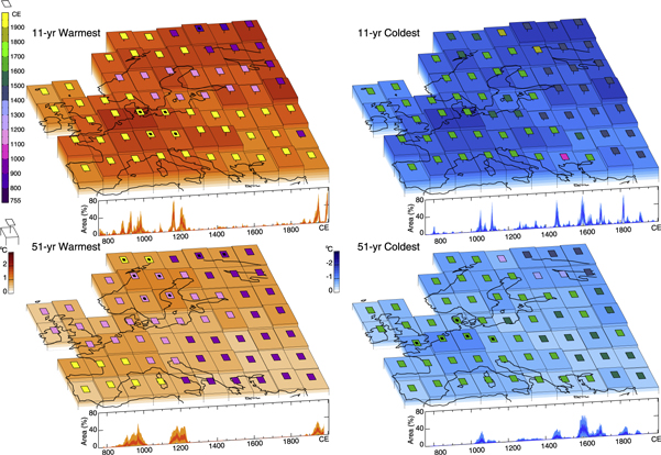
Figure 2. Top left: spatial distribution, magnitude and extension of the warmest 11 yr periods in European summer temperature. Grid cell height represents the ensemble mean temperature anomaly (in °C, with respect to 755–2003 CE) and the shading is incremented with a contour interval of +0.2 °C. The colour and the height of the squared symbols above each grid point identify the most likely date and the temperature uncertainty (+2·SD level) of the warmest mean 11 yr period across the ensemble, respectively. Dots in squares denote those grid points with more than 75% of the ensemble members agreeing on the timing of the warmest 11 yr period (i.e. having their warmest 11 yr periods in the same 100 yr interval). The front panel of the map shows the ensemble-based temporal evolution of the fraction of European surface (in % of total analysed area) with 11 yr mean summer temperatures exceeding their +2 SD from the 755–2003 CE mean climatology. The light (dark) red shading indicates the 5th–95th percentile (±0.5·SD) range of the ensemble distribution. Bottom left: as in the top left panel but for 51 yr mean periods. Right: as left panels, but for the 11 yr (top) and 51 yr (bottom) coldest periods. See SOM for details.
Download figure:
Standard image High-resolution imageJoint evaluation of reconstructions and AOGCM simulations covering the period 850–2000 CE allows for comparative assessments of these two independent sources of information of past climate variability. It further provides insights into the relative contributions of estimated external forcing and internal dynamics. For both the SUNWIDE and SUNNARROW solar variability sub-ensembles, figure 3 shows the ensemble average and the 10, 25, 75 and 90 percentiles. Purple and green shading in figure 3 represent measures of the overlap among the ensemble of simulations, taking into account the uncertainty due to internal climate variability. The overlap was calculated according to Jansen et al (2007). The scores are summed over all simulations and scaled to add one for a given year. The simulated range of internal variability is ideally estimated based on SD from long control simulations with constant external forcing, however, these were not available for all models. Therefore, SDs were estimated from the high-pass (51 yr) filtered temperature outputs of the forced simulations. The attribution of climate response to external forcing in the multi-model ensemble is complicated by the heterogeneous choices of forcing agents (table S14). For example, some pre-PMIP3 simulations did not include anthropogenic aerosols or orbital forcing. With this caution in mind, the mean European temperature reconstructions using BHM and CPS correlate with the SUNWIDE ensemble (r = 0.61, p < 0.05, accounting for serial autocorrelation; figure 3) as well as with the SUNNARROW ensemble mean (r = 0.55 and 0.57 for BHM and CPS, respectively, both at p < 0.05). Reconstructed cold conditions (mid-13th, mid-15th, and early 19th century) at multi-decadal time-scales mostly agree with simulated temperature minima attributed to solar and volcanic forcing (Hegerl et al 2011). The reconstructed minima at the beginning of the 12th century and around 1600 CE have no counterpart in the climate model data (figure 3), suggesting either an important role of internal variability (Goosse et al 2012b) or inaccuracies in model forcing (Fernández-Donado et al 2013, 2015). An alternative interpretation of the discrepancies as being related to shortcomings in the reconstructions is unlikely due to considerable support for these temperature minima from other NH proxy evidence. Colder conditions in the decades around 1100 CE were also observed in other parts of the world, e.g. Russian plains (Klimenko and Sleptsov 2003, SOM, figure S9), East China (Ge et al 2003), the Tibetan Plateau (Thompson et al 2003, Liu et al 2006) and the Eastern Canadian Arctic (Moore et al 2001). Glacier advances are reported around this time for the Alps, Western Canada, the Canadian Arctic, Greenland, the Tibetan Plateau, and the Antarctic Peninsula (for a review, see Solomina et al 2015). Additionally, proxy-based evidence supports the cold conditions of the 16th–17th centuries (figure S9). Local proxy records of various types (see figure 2 in Christiansen and Ljungqvist 2012), inferences of glacier expansions around the world (e.g. Solomina et al 2015), continental multi-proxy reconstructions (e.g. PAGES 2k Consortium 2013), and extra-tropical NH tree-ring based summer temperature reconstructions (Briffa et al 2004, Masson-Delmotte et al 2013 and references therein; Schneider et al 2015, Stoffel et al 2015) support the existence of a strong and geographically widespread very cold episode around 1600 CE.

Figure 3. Simulated and reconstructed European summer land temperature anomalies (with respect to 1500–1850 CE) for the last 1200 yr, smoothed with a 31 yr moving average filter. BHM (CPS) reconstructed temperatures are shown in blue (red) over the spread of model runs. Simulations are distinguished by solar forcing: stronger (SUNWIDE, purple; TSI change from the LMM to present >0.23%) and weaker (SUNNARROW, green; TSI change from the LMM to present <0.1%). The ensemble mean (heavy line) and the two bands accounting for 50% and 80% (shading) of the spread are shown for the model ensemble (see SOM for further details).
Download figure:
Standard image High-resolution imageIn agreement with the results of Hegerl et al (2011) using temperature reconstructions from Luterbacher et al (2004), our findings suggest that changes in external forcing have had a pronounced influence on past European summer temperature variations. A more in-depth detection and attribution analysis of temperature changes over Europe, as well as those over other PAGES 2k regions (PAGES 2k Consortium 2013) can be found in PAGES2k-PMIP3 Group (2015). The marginally better agreement with the SUNWIDE ensemble lends tentative support to both the importance of changes in solar forcing in driving continental past climate variations as well as a potentially greater role for solar forcing in driving European summer temperatures than is currently present in the CMIP5/PMIP3 simulations. This might be evidence for an enhanced sensitivity to solar forcing in this particular region due to dynamics, as has been suggested by modelling studies (see e.g. Ineson et al 2015). However, this is beyond the current scope of this paper. It should also be noted, that most periods with anomalously low solar activity during the last millennium coincide with clustering of medium-to-strong tropical volcanic eruptions, thus complicating a clear separation of individual forcing contributions to large-scale temperature variations (Zanchettin et al 2013a, Schurer et al 2014).
The European summer temperature response to strong tropical volcanic events is analysed through Superposed Epoch Analysis (SEA, e.g. Fischer et al 2007, Hegerl et al 2011) for the PMIP3 model simulations and the BHM reconstructions (figures S13–S14). For each volcanic forcing, the 12 strongest volcanic events are selected, following the same approach as in PAGES2k-PMIP3 group (2015). The SEA for the reconstruction is performed for the 13 strongest tropical volcanic eruptions (> =VEI 5) published in Esper et al (2013). The selected eruptions all occurred during the time period covered by the gridded BHM reconstruction (figure S14). We show the anomalies during the year of the eruptions and the 3 yr delayed post-eruption anomalies evaluated with respect to the pre-eruption climatology, defined as the average state over the five summers preceding the eruption. Using the PMIP3 climate models the multi-model response after the strongest volcanoes over the last millennium shows an overall European summer cooling (figure S13), though much stronger than in the reconstructions (figure S14) and peaking during the year of the eruption and the first year thereafter. The composite analysis from the reconstructions clearly reveals that the European summer cooling is strongest in the first and second year after the eruptions. The average anomalies are of the order of 0.5 °C.
The summer cooling is confirmed by a separated analysis for a selection of strong tropical (Samalas 1257, Huaynaputina 1600, Parker 1641 and Tambora 1815) and non-tropical (Laki 1783/1784) eruptions (figure S15, Lavigne et al 2013, Sigl et al 2015, Stoffel et al 2015) in the BHM reconstructions.
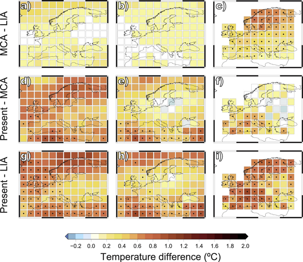
Patterns of past sub-continental climate variability contain information about the influence of external factors that affect the climate system and, together with climate models, can be used to better understand how internal dynamics contribute to determining the regional climate response to external forcing. Figure 4 shows the spatial differences between the MCA, LIA, and present-day averages for simulated and reconstructed European summer temperatures. Note that the following results do not differ significantly if alternative definitions of periods are chosen (not shown). Overall, simulated differences are statistically significant at the 5% level only at a few grid-points, even without correction for multiple testing, and are not clearly consistent across the model ensemble (figure 4). The models tend to simulate the largest changes for all the three periods over Northern Europe, resembling the typical pattern of temperature response to changes in forcing (e.g. Zorita et al 2005) and the possible signature of Arctic amplification (see Masson-Delmotte et al 2013). While the simulated pattern for both model groups qualitatively matches the reconstruction of the MCA to LIA transition, its amplitude is smaller (figures 4(a)–(c)) for both sub-ensembles. The differences between the reconstructed spatial patterns averaged during the MCA and the present day (figure 4(f)) are distinct from the same simulated metric (figures 4(d) and (e)), particularly over North–Eastern Europe. The reconstructed MCA is slightly warmer than recent decades in many parts of (primarily) Northern and Eastern Europe, while the simulations reveal a more generalised and warmer present day over the whole spatial domain (figures 4(d)–(f)), with the SUNNARROW simulations appearing closer to the reconstructions than SUNWIDE. Also the SUNNARROW ensemble fails to fully reproduce the magnitude of the reconstructed temperature differences between the LIA and present day (figures 4(g)–(i)) for which the agreement between different simulations is regionally limited to Southern and Western parts of the target region.
Figure 4. Simulated and reconstructed summer (June–August) temperature differences for three periods: (a), (b), (c) MCA (900–1200 CE) minus LIA (1250–1700 CE); (d), (e), (f) present (1950–2003 CE) minus MCA; and (g), (h), (i) present minus LIA. Model temperature differences (left and central columns) indicate average temperature changes in the ensemble of available model simulations (see table S13). Model simulations are grouped into SUNWIDE (TSI change from the LMM to present >0.23%; left column) and SUNNARROW (TSI change from the LMM to present <0.1%; middle column). Reconstructed temperature differences with the BHM method are shown in the right column. Simulations have been weighted by the number of experiments considered from each model. Dots indicate significant (p < 0.05) changes in the reconstruction; in the simulation ensemble a dot indicates at least 80% of agreement in depicting significant (p < 0.05) changes of the same sign.
Download figure:
Standard image High-resolution image
If we assume the BHM reconstruction to be our best available evidence regarding the MCA–LIA transition, the amplitude mismatch between the multi-model ensemble and the reconstructions suggest either a reduced model sensitivity, or an underestimation of model forcings, or that internal variability may play a dominant role. Alternatively a combination of all these factors may be at play. The fact that different simulations agree with each other only in a limited part of the domain indicates a hint that the response to forcing can be model-dependent and that ensemble members may diverge depending on initial and boundary conditions (Zanchettin et al 2013b). Concerning the latter, changes in ocean circulation may be important, including aspects of variability such as the state of the Atlantic Multidecadal Oscillation (AMO; Kerr 2000, Alexander et al 2014) and dynamical implications of phasing between the AMO and North Pacific sea-surface temperatures for hemispheric-scale teleconnections (i.e. Zanchettin et al 2013a). Additionally, some of the models may not be able to reproduce the dynamical mechanisms shaping the regional responses to forcing variations (e.g. Ineson et al 2015), owing to, for example, a lack of horizontal resolution or the absence of a well-resolved stratosphere (Mitchell et al 2015).
Conclusions and outlook
In this study, we have updated and extended reconstructions of European summer temperature variation for the CE using a suite of proxy records and a BHM approach. We also jointly analysed the new summer temperature reconstruction with several state-of-the-art reconstructions and AOGCM simulations in order to clarify the relative role of external forcing and internal variability for the evolution of European summer temperatures at different spatial and temporal scales. Reconstructions of mean European summer temperatures compare well for both the CPS and the BHM methods, strengthening our confidence in the derived results. Our European summer temperature reconstructions compare well with independent instrumental and lower resolution proxy-derived temperature estimates but show larger amplitudes in summer temperature variability than previously reported. There is thus merit in further studies combining instrumental series with low and high-resolution summer temperature proxies in a Bayesian hierarchical framework (Werner and Tingley 2015). Our primary findings indicate that the 1st and 10th centuries CE could have experienced European mean summer temperatures slightly but not statistically significantly (5% level) warmer than those of the 20th century. However, summer temperatures during the last 30 yr (1986–2015) have been anomalously high and we find no evidence of any period in the last 2000 years being as warm (tables S11, S12). The anomalous recent warmth is particularly clear in Southern Europe where variability is generally smaller, and where the signal of anthropogenic climate change is expected to emerge earlier (e.g. Mahlstein et al 2011). European summer mean temperatures appear to reflect the influence of external forcing during periods with sustained sub-decadal (volcanic) and multi-decadal (volcanic, solar, GHG) changes. Reconstructed summer temperature anomalies for the Roman period and MCA in Europe, which are not reflected to the same extent in large-scale means have important implications for predicting the magnitude and frequency of extremes. Our results show that subcontinental regions may undergo multi-decadal (and longer) periods of sustained temperature deviations from the continental average indicating that internal variability of the climate system is particularly prominent at sub-continental scales, in accordance with results from simulations of future anthropogenic-driven climate change (Deser et al 2012). The new reconstructions provide the basis for future comparison with extended simulations beyond the last millennium that are currently underway. A significant advantage of the gridded reconstructions is that they will allow an in-depth analysis of the spatial co-variability within the European realm in comparison to higher resolution climate simulations capable of mimicking the complex geographical and climatic structure of Europe. Further, forcings such as volcanic aerosols, solar and land-use change are expected to have unique fingerprints of temperature change, potentially affecting some areas of Europe more than others. In future analyses we will use the long-timescale sub-continental information presented here to try to disentangle these different factors from internal variability.
Acknowledgments
Support for PAGES 2k activities is provided by the US and Swiss National Science Foundations, US National Oceanographic and Atmospheric Administration and by the International Geosphere-Biosphere Programme. JPW acknowledges support from the Centre of Climate Dynamics (SKD), Bergen. The work of OB, SW and EZ is part of CLISAP. JL, SW, EZ, JPW, JGN, OB also acknowledge support by the German Science Foundation Project 'Precipitation in the past millennia in Europe–Extension back to Roman times'. MB acknowledges the Catalan Meteorological Survey (SMC), National Programme I + D, Project CGL2011-28255. PD and RB acknowledge support from the Czech Science Foundation project no. GA13-04291S. VK was supported by Russian Science Foundation (grant 14-19-00765) and the Russian Foundation for Humanities (grants 15-07-00012, 15-37-11129). GH and AS are supported by the ERC funded project TITAN (EC-320691). GH was further funded by the Wolfson Foundation and the Royal Society as a Royal Society Wolfson Research Merit Award (WM130060) holder. NY is funded by the LOEWE excellence cluster FACE2FACE of the Hessen State Ministry of Higher Education, Research and the Arts; HZ acknowledge support from the DFG project AFICHE. Lamont contribution #7961. The reconstructions can be downloaded from the NOAA paleoclimate homepage: www.ncdc.noaa.gov/paleo/study/19600. LFD, EGB and JFGR were supported by grants CGL2011-29677-c02-02 and CGL2014-599644-R. All authors are part of the Euro-Med 2k Consortium.