

Abstract
Carbon dioxide removal (CDR) approaches are efforts to reduce the atmospheric CO2 concentration. Here we use a marine carbon cycle model to investigate the effects of one CDR technique: the open ocean dissolution of the iron-containing mineral olivine. We analyse the maximum CDR potential of an annual dissolution of 3 Pg olivine during the 21st century and focus on the role of the micro-nutrient iron for the biological carbon pump. Distributing the products of olivine dissolution (bicarbonate, silicic acid, iron) uniformly in the global surface ocean has a maximum CDR potential of 0.57 gC/g-olivine mainly due to the alkalinisation of the ocean, with a significant contribution from the fertilisation of phytoplankton with silicic acid and iron. The part of the CDR caused by ocean fertilisation is not permanent, while the CO2 sequestered by alkalinisation would be stored in the ocean as long as alkalinity is not removed from the system. For high CO2 emission scenarios the CDR potential due to the alkalinity input becomes more efficient over time with increasing ocean acidification. The alkalinity-induced CDR potential scales linearly with the amount of olivine, while the iron-induced CDR saturates at 113 PgC per century (on average  PgC yr−1) for an iron input rate of 2.3 Tg Fe yr−1 (1% of the iron contained in 3 Pg olivine). The additional iron-related CO2 uptake occurs in the Southern Ocean and in the iron-limited regions of the Pacific. Effects of this approach on surface ocean pH are small
  .
.
Export citation and abstract BibTeX RIS

Original content from this work may be used under the terms of the Creative Commons Attribution 3.0 licence. Any further distribution of this work must maintain attribution to the author(s) and the title of the work, journal citation and DOI.
1. Introduction
Humans perturb the CO2 concentration in the atmosphere by burning of fossil fuels and by land use change. CO2 is a greenhouse gas and its accumulation in the atmosphere leads to a warming of the Earth system, and to changes in all parts of the climate system, e.g. the hydrological cycle. About a quarter of the annual CO2 emissions is taken up by the ocean (Le Quéré et al 2015), leading to acidification with potentially detrimental effects for ocean ecosystems and their services to humans (Pörtner et al 2014).
Most IPCC emission scenarios project a warming of more than 2 °C compared to pre-industrial levels by the end of the 21st century (IPCC 2013, Rogelj et al 2015), hence a large effort is needed to keep the temperature rise below the agreed-upon threshold of 2 °C (UNFCCC 2009). To stay below this threshold, zero and net negative emissions might be necessary from 2060 onwards (Rogelj et al 2015). Owing to this necessity, besides taking action to reduce carbon emissions, two types of geoengineering methods have been proposed to counteract global warming. Albedo modification (or 'solar radiation management') is considered a 'quick-fix' that could counteract the warming on the time-scale of years at relatively low cost (Kravitz et al 2011, National Research Council 2015). However, its side-effects are poorly understood and applying albedo modification at global scale would lead to regional impacts, such as further changes in precipitation patterns (Kravitz et al 2013, National Research Council 2015). Albedo modification might cool the planet. As side effects of these approaches the carbon cycle might also be influenced, potentially leading to large variations in atmospheric CO2, e.g. a cooler ocean might store more CO2 (Oschlies et al 2010b, Keller et al 2014), temperature and precipitation changes on land might impact the terrestrial carbon cycle (Oschlies et al 2010b, Kravitz et al 2013, Glienke et al 2015). A termination of the albedo modification measure would lead to a large and sudden temperature rise (Jones et al 2013). The second type of geoengineering approaches are carbon dioxide removal (CDR) methods which directly address the cause of climate change. As atmospheric CO2 would be lowered by CDR methods, carbon from natural ocean and land sinks would degas until a new equilibrium is established. Due to this rebound effect, not only the accumulated anthropogenic CO2 in the atmosphere, but about twice this amount of CO2 has to be removed from the atmosphere for any intended atmospheric CO2 reduction (e.g. 42 Gt of carbon needs to be removed from the system to reduce atmospheric CO2 by 10 ppmv or 21 GtC) (Cao and Caldeira 2010a, Matthews 2010).
One such CDR method is enhanced weathering (or dissolution) of silicate rocks (Hartmann et al 2013). On geological time-scales, natural weathering will be the ultimate sink for anthropogenic CO2 emissions (Archer 2005). An abundant magnesium silicate which dissolves in contact with CO2 and water is olivine ((Mg,Fe)2SiO4, Schuiling and Krijgsman 2006):

The reaction products, bicarbonate, silicic acid and Mg and Fe are transported to the oceans following the dissolution on land. Carbon is sequestered in the ocean in the form of bicarbonate and the increase of alkalinity leads to an increase of pH and further enhances the CO2 uptake capability of the ocean (Köhler et al 2010). Direct open ocean dissolution of olivine additionally stimulates biological production and CO2 sequestration due to the fertilising effect of the additional silicate (Köhler et al 2013). Olivine also contains iron which is a limiting micronutrient for phytoplankton production in extended ocean regions, such as the Southern Ocean (De Baar et al 1995, Smetacek et al 2012), the subpolar North Pacific (Martin and Fitzwater 1988), and large parts of the South Pacific (Behrenfeld et al 2009). However, the impact of iron fertilisation (a proposed CDR method of its own, Zeebe and Archer 2005, Aumont and Bopp 2006, Smetacek et al 2012) during open ocean dissolution of olivine was not quantified in previous studies.
The fraction of iron that goes into solution when lithogenic material such as dust is deposited in seawater varies between 0.01% and 80%, depending on a variety of factors that are not completely understood, such as mineralogy, chemical processing during atmospheric transport, wet versus dry deposition, and the concentration of organic iron-binding ligands in seawater (Baker and Croot 2010). Compared to other iron-containing minerals such as iron-oxyhydroxides, olivine is expected to dissolve more readily, so that we could expect the fraction of iron dissolved to be on the higher side. However, due to the low solubility of iron in seawater (Liu and Millero 2002) some of the iron from olivine is likely to quickly form iron-oxyhydroxide colloids and be scavenged onto available particles (Honeyman and Santschi 1989, Rose and Waite 2007). The degree to which this will happen depends also on whether the concentration of iron after dissolution of olivine exceeds that of organic iron-binding ligands present in seawater (Fishwick et al 2014), which is typically on the order of one to a few nmol l−1 in open oceans. The fraction of iron from olivine that ultimately becomes bioavailable is therefore hard to estimate at this point without further experimentation and thus we will explore a range of values (sensitivity analysis).
In this study, we aim to quantify the potential impact of iron fertilisation on the efficiency of olivine dissolution as a CDR method on a centennial time-scale, as well as its effects on primary production, carbon export and the abundance of phytoplankton functional types. We particularly strive to assess the sensitivity of CDR efficiency to the fraction of iron in olivine that becomes dissolved and stays long enough in solution to become bioavailable (which for brevity we call 'availability' in the following).
2. Model and numerical experiments
We use the marine regulated ecosystem and biogeochemistry model REcoM2 (Hauck et al 2013) coupled to the Massachusetts Institute of Technology general circulation model (MITgcm, Marshall et al 1997, MITgcm Group 2015). This model was also used in our previous study on the open ocean dissolution of olivine (Köhler et al 2013).
The model is configured globally without the Arctic Ocean. The resolution is 2° in longitude and 1/3 to 2° in latitude with higher resolution around the equator and in the Southern Hemisphere where the latitudinal resolution is scaled by the cosine of the latitude. The model has 30 depth levels and the vertical resolution decreases from 10 m at the surface to 500 m in the deep ocean.
The ecosystem model REcoM2 (Hauck et al 2013) carries 21 tracers, including the dissolved inorganic nutrients nitrate, silicic acid and iron. The intracellular pools of carbon, chlorophyll, nitrogen, silicon and CaCO3 for the two phytoplankton groups, diatoms and nanophytoplankton, are explicitly modelled and allow for dynamic intracellular stoichiometry, following Geider et al (1998). Detrital carbon, nitrogen, silicon and calcium carbonate are actively advected until degradation or remineralisation occurs.
The model has undergone some development since the study of Hauck et al (2013). Besides updating the MITgcm to the latest version (checkpoint 65n), the intracellular iron pool was made dependent on nitrogen (fixed Fe:N instead of Fe:C) as iron is physiologically rather linked to enzyme formation, especially the photosynthetic electron transport chain (Raven 1988, Behrenfeld and Milligan 2013) than to overall biomass that also includes carbohydrates and fatty acids. Furthermore, we included sedimentary sources of iron and we increased the ligand stability constant to 200  mol−1 and the iron solubility from 1% to 2%. The maximum chlorophyll to nitrogen ratio was set to 3.78 mg Chl (mmol N)−1 and the diatom chlorophyll degradation rate to 0.1 d−1.
The model is spun-up from 1900 to 1999 and we start the addition of olivine in the model year 2000 and run the model for 100 years (2000–2099). The model is forced with the normal year atmospheric forcing fields from the coordinated ocean research experiments (Large and Yeager 2009) during the spin-up and experimental period. Atmospheric CO2 is prescribed by a spline-fit to ice-core data (Enting et al 1994) until 1957, by the annually averaged Mauna Loa CO2 data after 1958 (Keeling et al 2009), and follows RCP8.5 from 2010 until 2099 reaching more than 900 ppm at the end of the century (Meinshausen et al 2011, van Vuuren et al 2011). Prescribing atmospheric CO2 is a simplification that underestimates sea-to-air back fluxes. Together with the omission of resulting variations in land carbon pools, this might lead to an overestimation of the CDR potential of the analysed approach that is dependent on the emission scenario (Oschlies 2009). As our model set-up uses climatological atmospheric forcing, we consider the effect of increasing atmospheric CO2 over that time period but no effects of climate change, such as warming and circulation changes. This setup has the advantage that the changes in biological production caused by olivine dissolution are rather independent from the chosen emission scenario. The disadvantage of this approach is that synergies between olivine dissolution and warming/circulation effects are omitted, however, we consider them to play only a secondary role.
We perform one control (CTRL, see table 1) simulation without addition of olivine, in all other simulations we add dissolved olivine to the surface ocean. Since this study is a follow-up of our previous analysis (Köhler et al 2013) we use the same dissolution scenario of 3 Pg of olivine per year. This choice is also supported by our previous finding that the alkalinity and silicic acid induced CDR potential scale linearly with the amount of dissolved olivine and by the fact that present day coal production (the largest global mining activity) was ∼8 Pg in year 2013 (International Energy Agency 2014), making a significantly larger annual olivine production over a short time rather unlikely. The olivine is assumed to dissolve immediately and completely and is spread uniformally throughout the year and over the entire surface ocean (standard scenario in Köhler et al 2013). In doing so, we aim for estimating the potential or upper limit of the approach. The importance of grain size, mixed layer depth, and sea surface temperature on the dissolution rates of olivine have already been discussed together with related energy costs in Köhler et al (2013) and is not repeated here. Assuming immediate and complete dissolution of olivine is thus an effort to estimate the maximum effects or the overall potential of the approach. Besides the control run, we perform model simulations in which we consider only the effects of alkalinity (ALK), and the joint effects of silicic acid and alkalinity but no iron (SI+ALK) from olivine dissolution. These two simulations are described in detail in Köhler et al (2013), but are repeated here to monitor the system response over 100 years in the modified model set-up.
Table 1. Model simulations. In all olivine dissolution experiments, 3 Pg of olivine are dissolved per year for the years 2000–2099. In the simulations with termination effect, olivine addition is stopped after 10 years.
| Short name | Description |
|---|---|
| CTRL | Control simulation, no olivine dissolution |
| ALK | Only alkalinity |
| SI+ALK | Silicic acid and alkalinity |
| FE_1 | Only iron effect, 1% Fe-availability |
| SI+ALK+FE_0.1 | Silicic acid, alkalinity and iron, 0.1% Fe-availability |
| SI+ALK+FE_1 | Silicic acid, alkalinity and iron, 1% Fe-availability |
| SI+ALK+FE_10 | Silicic acid, alkalinity and iron, 10% Fe-availability |
| SI+ALK+FE_100 | Silicic acid, alkalinity and iron, 100% Fe-availability |
| ALK_T | Only alkalinity, with termination effect |
| SI+ALK+FE_1T | Silicic acid, alkalinity and iron, 1% Fe-availability, with termination effect |
The sensitivity of carbon removal efficiency by olivine dissolution to iron solubility, scavenging and colloid formation is assessed by four model simulations in which silicic acid, alkalinity and iron are simultaneously released from olivine with iron availabilities of 0.1%, 1%, 10%, and 100% (SI+ALK+FE_X, where X describes the availability of iron). Olivine is assumed to have a molar weight of 147 g mol−1 and a Mg:Fe molar ratio of 9:1 typically found in nature (De Hoog et al 2010). Specifically, following equation (1), we increase alkalinity by 4 mol, silicate by 1 mol and iron by 0.2 mol per mol of olivine dissolved. The total amount of added iron is 0.23 Tg yr−1 in the 0.1% availability case. This is approximately the same number as the bioavailable iron input by dust (Mahowald et al 2005).
We also conduct two experiments to explore the termination effect of olivine input. In the termination experiments, we dissolve olivine for ten years and continue the model run for another 90 years without olivine dissolution. The termination experiments are conducted for the case where only alkalinity is considered (ALK_T) and for the case of joint consideration of alkalinity, silicic acid and iron with an Fe-availability of 1% (SI+ALK+FE_1T).
Furthermore, we conduct an additional simulation for the 1% availability case, where we only consider the addition of iron (FE_1), without increasing silicic acid and alkalinity, to investigate whether there are synergistic effects by simultaneously adding iron and silicic acid. Table 1 contains an overview of the performed simulation scenarios.
3. Results and discussion
Model results without olivine dissolution were published elsewhere (Hauck et al 2013, Köhler et al 2013, Hauck and Völker 2015). The model has changed slightly, hence we show global maps of mean export production, diatom, nanophytoplankton and total net primary production (NPP), pH and CO2 flux in the first ten years of the CTRL simulation and the temporal evolution of the surface iron concentration in the supplement (figures S2 and S3). The results of the mean state do not differ significantly from the previous version and we therefore refer the reader to the main text and supplement of Hauck et al (2013) and Köhler et al (2013) for further information. In the following we restrict our analysis to anomalies in the carbon cycle obtained from the assumed olivine dissolution.
3.1. Simulation of iron fertilisation within the concept of open ocean olivine dissolution
The additional consideration of iron fertilisation amplifies the alkalinity- and silicate-based CDR of olivine dissolution, leading to further increase of the potential oceanic CO2 uptake, NPP and export production (figure 1, table 2).
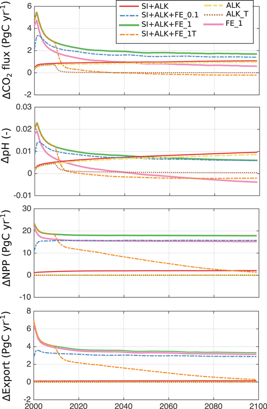
Figure 1. Timeseries of CO2 flux, pH, NPP and export production in different olivine dissolution scenarios relative to the control run. See table 1 for the list of simulations. Note that SI+ALK+FE_10 and SI+ALK+FE_100 are not shown for reasons of readability as they overlay the SI+ALK+FE_1 line.
Download figure:
Standard image High-resolution imageTable 2. Marine CO2 uptake (FCO2), pH, export production, total, nanophytoplankton and diatom net primary production (NPP, NPPS and NPPD, respectively) in the CTRL, in the SI+ALK simulation and in the simulations with iron availability varying between 0.1% and 10%. Numbers are means over the last ten years (2090–2099) of the simulation and in all experiments 3 Pg of olivine per year are dissolved. All units are PgC yr−1, except pH which is unitless. T stands for the run with the termination effect.
| CTRL | ALK | SI+ALK | SI+ALK+FE | ||||
|---|---|---|---|---|---|---|---|
| 0.1% | 1% | 1% T | 10% | ||||
| Global | |||||||
| FCO2 | 6.0 | 7.0 | 7.1 | 7.5 | 7.7 | 5.8 | 7.8 |
| pH | 7.746 | 7.754 | 7.755 | 7.752 | 7.752 | 7.744 | 7.752 |
| Export | 10.2 | 10.2 | 10.4 | 13.1 | 13.5 | 10.6 | 13.6 |
| NPP | 40.4 | 40.4 | 42.5 | 56.2 | 58.3 | 42.1 | 58.5 |
| NPPS | 22.4 | 22.4 | 19.2 | 29.2 | 29.1 | 23.4 | 29.0 |
| NPPD | 18.1 | 18.1 | 23.3 | 27.0 | 29.2 | 18.6 | 29.4 |
| South of 40°S | |||||||
| FCO2 | 2.5 | 2.7 | 2.8 | 3.1 | 3.4 | 2.5 | 3.4 |
| pH | 7.732 | 7.737 | 7.738 | 7.736 | 7.736 | 7.730 | 7.736 |
| Export | 2.9 | 2.9 | 2.9 | 3.8 | 4.2 | 3.0 | 4.2 |
| NPP | 7.2 | 7.2 | 7.4 | 9.8 | 11.8 | 7.4 | 11.9 |
| NPPS | 1.6 | 1.6 | 1.3 | 1.9 | 1.9 | 1.8 | 1.9 |
| NPPD | 5.5 | 5.5 | 6.2 | 7.9 | 9.9 | 5.6 | 10.0 |
In the last decade of the simulation scenarios, the total effect of olivine dissolution with the 0.1% (1%) iron availability scenario leads to an additional CO2 uptake of 1.4 PgC yr−1 (1.6 PgC yr−1) or a rise by +24% (+28%) compared to the CTRL. The relative contributions of alkalinity, silicic acid and iron in the 0.1% (1%) scenario amount to 69% (57%), 7% (6%) and 24% (37%), respectively. The effect of iron fertilisation saturates already at an availability of 1% with a maximum in Fe-driven CO2 uptake of 0.6 PgC yr−1 or 0.2 PgC per Pg olivine in the last ten years of the simulation (figure 1(a)).
The annual mean pH is 0.006 units higher than in CTRL at the end of the olivine dissolution simulation with 0.1% Fe-availability. The effects of alkalinity (0.009) and silicic acid (0.001) lead to a larger pH restoration, however, the iron effect leads to an increase of pH initially, but to a decrease of pH after approximately 50 years when the transport of remineralised carbon reaches the surface and outweighs the current carbon draw-down by iron fertilisation (figure 1(b)). A termination of the open ocean dissolution of olivine results in a lower pH relative to the unperturbed CTRL state only 10 years after the termination. The pH increase due to olivine dissolution is small compared to the pH decrease driven by anthropogenic carbon uptake from about 8.1 to  7.8 in our simulations over the 21st century.
Diatom NPP increases by 9.0 PgC yr−1 or 50% after 100 years in the low (0.1%) Fe-availability scenario. Here, silicic acid contributes 58% and Fe-fertilisation 42% to the total rise in diatom NPP. Diatom primary production can be increased by a maximum of 11 PgC yr−1 by olivine addition when an Fe-availability ≥1% is assumed (figure 2(b)). Nanophytoplankton NPP simultaneously increases by 6.8 PgC yr−1 or 30% and saturates already at 0.1% iron availability (table 2, figure 2(b)). In total, the enhancement of NPP through the input of silicic acid and iron as biproducts of the olivine dissolution amount to +39% or +15.7 PgC yr−1 in the 0.1% availability scenario and to +45% or +18.0 PgC yr−1 in the 1% availability scenario with a relative contribution of ∼90% from iron (figures 1(c), 2(a)).
While silicic acid favours a shift towards diatoms (see table 2 and Köhler et al 2013), iron stimulates NPP of both diatoms and nanophytoplankton (figures 2 and 3 and Aumont and Bopp 2006).
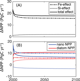
Figure 2. Effect of olivine dissolution on NPP: time-series of (A) total, (B) diatom (red) and nanophytoplankton (blue) NPP in the SI+ALK+FE_1 simulation relative to the CTRL simulation (full line) and the contributions of iron (dashed line) and silicic acid (dotted line) fertilisation effects.
Download figure:
Standard image High-resolution image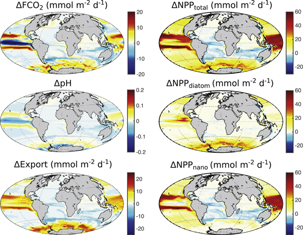
Figure 3. Effects of iron during olivine dissolution on CO2 flux (FCO2, positive: into ocean, mmol m−2 d−1), pH, export production (mmol m−2 d−1), total, diatom and nanophytoplankton NPP (all mmol m−2 d−1) in the last ten years of the simulation with 3 Pg olivine dissolution and 1% iron availability (SI+ALK+FE_1), relative to the SI+ALK simulation.
Download figure:
Standard image High-resolution imageIn the last ten years of the simulation, diatom NPP changes based on Fe fertilisation are strongest in the Southern Ocean and in the equatorial and North Pacific, and close to zero in the remaining ocean basins. Nanophytoplankton NPP thrives outside the areas where diatoms profit: in a band to the North of the Southern Ocean and in the whole Pacific except the equatorial East Pacific (figure 3). Nanophytoplankton NPP is reduced in the Atlantic Ocean and in the subtropical Indian Ocean where iron is not the most limiting nutrient in the CTRL simulation (figure 4). The largest increase in CO2 uptake is in the Southern Ocean and in a band north and south of the eastern equatorial upwelling area in the Pacific with minor contributions from the north Pacific and north Atlantic. In the eastern equatorial upwelling area itself a strong decrease of CO2 uptake is detected (figure 3).

Figure 4. The most limiting nutrient for diatom (left) and nanophytoplankton (right) growth in the CTRL (top) and SI+ALK+FE_1 (bottom) simulations, average over 2090–2099. When no limitation factor is below 0.7, we assume that nutrients are not limiting, but rather light or temperature.
Download figure:
Standard image High-resolution imageGlobally, the export production of particulate organic matter at 100 m water depth increases by 2.9 PgC yr−1 (+28%) at the end of the 100 years simulation (0.1% Fe-availability) with a dominance of the iron fertilisation effect (+2.7 PgC yr−1) over that of silicic acid fertilisation (0.2 PgC yr−1). At maximum an additional export of 3.3 PgC yr−1 can be obtained by olivine dissolution for an availability of iron of 1% or more (table 2, figure 1(d)).
The largest effects of iron fertilisation by olivine dissolution occur within the first ten years of the simulations (figure 1). When terminating the continuous dissolution of olivine, the dominant part of the benefit of the larger oceanic CO2 uptake is lost within a few years and a state close to the control simulation without olivine addition is reached within approximately one decade (figure 1). Terminating open ocean dissolution of olivine dissolution leads to a lower pH relative to the CTRL simulation ten years after the termination (−0.002 in the last decade of the simulation) and to a loss of oceanic CO2 to the atmosphere relative to CTRL 25 years after the termination (−0.2 PgC yr−1 in the last decade of the simulation). However, the cumulative sum of CO2 uptake is at every time higher in the SI+ALK+FE_1T simulation than in the CTRL, indicating that the release of the remineralised carbon to the atmosphere is rather slow. Net primary and export production show a slower recovery to pre-olivine conditions and are still enhanced relative to the CTRL simulation at the end of the simulations.
Nearly all of the iron-effect on production, pH and CO2 flux occur in the Southern Ocean and in the Pacific (figure 3) where iron is the most-limiting nutrient in our CTRL simulation (figure 4). Despite the relatively short spin-up and a decreasing trend in global surface iron concentration (−6% over 100 years) that is caused by regions where iron is not a limiting nutrient (Atlantic and Indian Oceans), the surface iron concentrations in the Southern Ocean and in the Pacific vary little over time in the CTRL simulation and show no clear linear trend (figure S3). In addition, the surface iron perturbation by olivine dissolution is much larger than any temporal variability in these regions (figure S3). We can thus assume, that the response to iron addition does not change over time due to model drift. In the Pacific Ocean, models differ in the degree and extent of iron limited regions (Laufkötter et al 2015) and the response of primary production to iron addition will be model dependent. Traditionally, it is assumed that iron is the most limiting nutrient in high-nutrient-low-chlorophyll (HNLC) regions. Recent evidence, however, suggests that iron can also be a limiting factor in non-HNLC regions on a seasonal scale (e.g., Nielsdóttir et al 2009). Behrenfeld et al (2009) report strong evidence for iron (co-)limitation in large areas of the south Pacific Ocean.
The consumption of additional macronutrients along with the micronutrient iron in the Southern Ocean leads to nutrient depletion in Antarctic surface waters that get subducted to form northwards moving mode waters. The effects of this nutrient depletion become apparent only in the Atlantic and Indian Ocean in our model where NPP is reduced north of 40°S (figure 3). This is in line with the current understanding that the inefficiency of the biological carbon pump in the Southern Ocean due to the iron deficiency fuels present-day biological production in low latitudes (Sarmiento et al 2004). An enhanced efficiency of the biological carbon pump in the Southern Ocean therefore reduces NPP in lower latitude upwelling regions on multi-decadal to centennial time-scales (Rodgers et al 2003).
We also tested for synergistic effects of silicic acid and iron addition by comparing the iron effect in an iron-only scenario (FE_1) to the joint addition of iron with alkalinity and silicic acid (SI+ALK+FE_1). Synergistic effects favour diatom NPP, which is affected most strongly at the start of the simulation (+1.5 PgC yr−1), and decreases over time to about +0.7 PgC yr−1 in model year 2099 (figure S1). The simultaneous addition of silicic acid and iron has a negative effect on nanophytoplankton NPP (−1 PgC yr−1 in year 2000, −0.1 PgC yr−1 in year 2099). Synergistic effects on total NPP, export production and CO2 flux are about 0.6, 0.05 and 0.03 PgC yr−1 in year 2099, respectively, and are small in comparison to the iron effect itself.
All carbon fluxes saturate at an available iron input of 2.3 Tg Fe yr−1 (or a one-time per year increase of 1.1 nmol Fe L−1 in the upper 100 m; 1% Fe-availability scenario) in our set of simulations (figure 5(c)). The potential of carbon sequestration by olivine dissolution increases from 0.36 PgC per Pg olivine (SI+ALK) after 100 years to 0.57 PgC yr−1 per Pg olivine when considering the iron fertilisation effect with an availability of 1%.

Figure 5. (A) The temporal evolution of carbon sequestration potential of olivine assuming a 1% Fe-availability and the contributions of silicic acid, alkalinity and iron (1% availability). The alkalinity effect increases over time due to the higher sensitivity of dissolved CO2 to alkalinity perturbation in a high CO2 ocean, whereas the iron effect decreases over time due to the remineralisation of organic carbon and its transport to the surface. See text. (B) Ratio of ΔCO2 uptake to Δ export in full olivine dissolution scenarios (SI+ALK+FE) with varying Fe-availability relative to the SI+ALK simulation. Results for 1%, 10% and 100% Fe-availability overlay each other. (C) ΔCO2 flux (black, left axis), Δexport production (red, left axis) and ΔNPP (blue, right axis) for 3 Pg olivine dissolved, dependent on the total amount of iron that is released. Average over last ten years of model run (2090–2099). Note that Δexport at 0 Fe input is 0.07 PgC per Pg olivine (see SI+ALK in table 2). (D) The sensitivity of CO2 (aq) to an alkalinity addition of 1 mmol m−3 in the CTRL, ALK and SI+ALK+FE_1 simulations, that hardly differ.
Download figure:
Standard image High-resolution image
The carbon uptake potential after a century from alkalinity and silicic acid effects is larger than the 0.28 PgC per Pg olivine that was found after 10 years in Köhler et al (2013). This difference can be explained by the steady increase of the CO2 flux response to alkalinisation (32% increase to 0.33 PgC per Pg olivine from 2010 to 2099, figure 5(a)). We explain this temporal evolution of alkalinity-driven CO2 uptake by the increased sensitivity of CO2 (aq) and consequently CO2 flux to alkalinity and carbon perturbations in a high-CO2 ocean (Egleston et al 2010, Hauck and Völker 2015). We illustrate the four-fold increase of the sensitivity of CO2(aq) to alkalinity input over 100 years in figure 5(d). This sensitivity is calculated as

with  and with output from CO2SYS which is run with model fields of surface DIC, alkalinity, temperature, salinity, dissolved silicic acid and phosphate (converted from the modelled nitrate fields by the Redfield ratio).
  is defined according to Egleston et al (2010):

This rise in the CO2 uptake of the ocean due to the alkalinity input depends on the assumed changes in the anthropogenic emissions and would be smaller in other RCP scenarios with lower atmospheric CO2 concentrations.
The alkalinity effect on CO2 uptake due to olivine dissolution can be considered permanent in the sense that even after a termination, CO2 uptake will always be larger or equal to CTRL and the sequestered carbon will not be released to the atmosphere as long as alkalinity is not removed from the ocean. However, the iron effect of olivine addition is temporary, i.e. terminating an olivine dissolution experiment that releases significant amounts of iron would lead to a reduced CO2 uptake capacity after the termination, i.e. in our model the CO2 uptake is reduced relative to the CTRL simulation three decades after the termination (figure 1).
3.2. Discussing iron fertilisation
The CDR potential of iron fertilisation decreases over time from 1.6 to 0.2 PgC per Pg olivine (or from 4.8 to 0.6 PgC year−1). Our estimate of a total CO2 removal by iron fertilisation within one century of 113 PgC is almost twice as high as the 60 PgC obtained with the PISCES model in a study that explicitly simulates the ecosystem response to iron fertilisation (Aumont and Bopp 2006). Other studies that assumed complete macro-nutrient draw-down in simpler biogeochemical models gave higher numbers by design (e.g. 120–277 PgC Jin and Gruber 2003, Cao and Caldeira 2010b). Zeebe and Archer (2005) estimate a lower reduction of 30 PgC as they consider only 15 fertilisation events per year South of 55°S. When fertilising only the Southern Ocean for 92 years about 60 PgC (or 0.6 PgC yr−1) are taken up by the ocean in a study by Oschlies et al (2010a). The higher response in our model compared to Aumont and Bopp (2006) is partly due to larger areas of iron limitation in the Pacific Ocean in REcoM2 (figure 4). Models differ widely in the simulation of nutrient limitation in the Pacific (Laufkötter et al 2015), and recent evidence suggests that iron limitation could be more wide-spread than traditionally assumed based on macro-nutrient concentrations (Behrenfeld et al 2009, Nielsdóttir et al 2009). Aumont and Bopp (2006) use a lower limit for iron concentration of 0.01 nM to which iron is restored. In addition the models differ in the CO2 scenarios (RCP8.5 in REcoM2, SRES98-A2 in PISCES) and whether they prescribe atmospheric CO2 concentrations (REcoM2) or emissions (PISCES). The fact that REcoM2 prescribes concentrations and that we use a higher emission scenario can likely explain parts of the higher CO2 removal potential. Furthermore, the ecosystem models differ in various details, e.g. variable C:N but fixed Fe:N ratios in the version of REcoM2 used here, compared to fixed C:N and variable C:Fe ratios in PISCES.
Our model simulates an export efficiency of 20% (export at 100 m relative to vertically integrated NPP) independent of Fe-availability. This is slightly higher than the 17% reported by Aumont and Bopp (2006), but lower than the 50% sequestration efficiency (at 1000 m) that Smetacek et al (2012) observed in an open ocean iron fertilisation experiment, in which the formation of fast sinking diatom aggregates accelerated carbon transport to the deep ocean.
The ratio of ΔCO2 uptake to Δexport (relative to SI+ALK) decreases with time from approximately 85% at ≥1% Fe-availability (75% at 0.1% Fe-availability) to about 20% (12%) after 100 years (figure 5(b)) as expected due to remineralised carbon being transported back to the surface by the ocean circulation (Aumont and Bopp 2006). These numbers compare well with Aumont and Bopp (2006, 60% at start, 25% at end).
3.3. Feasibility and side-effects
Our study aims to estimate the carbon dioxide reduction potential (i.e. its upper limit) of the olivine dissolution approach by assuming total and instantaneous dissolution of the distributed olivine. Any real-world application of this approach might lead to a smaller molar ratio of oceanic CO2 uptake per dissolved olivine simply due to an incomplete dissolution of the material within the surface mixed layer (Köhler et al 2013).
The iron contained in olivine increases the CDR potential of olivine dissolution by roughly 60% (figure 5(a) + (c)). At least 28% of the additional NPP and 40% of the increase in export production occurs in the Southern Ocean (table 2). The relative dissolution rate of olivine depends on temperature and on the depth of the mixed layer. Although the deep mixed layers in the Southern Ocean might lead to long residence time of distributed particles in the surface ocean, the low temperatures likely lead to slow dissolution rates (Köhler et al 2013), and a large fraction of the particles would probably sink undissolved to the abyss. Olivine dissolution rates were not yet derived for polar conditions (e.g. Hangx and Spiers 2009, Rimstidt et al 2012). Köhler et al (2013) estimate relative olivine dissolution rates around 50% between 40 and 60°S and between 10% and 40% south of 60°S. Olivine dissolution rates from long-term laboratory experiments are an order of magnitude smaller than from shorter experiments due to the growth of a biotic community at the surface of the rock (Oelkers et al 2015). Dissolution kinetics estimated in Köhler et al (2013) might therefore be faster than what might be achievable in nature. In addition, there are few ships going to the Southern Ocean (Köhler et al 2013). Therefore a distribution of olivine from ballast water of ships of opportunity is only possible north of 40°S. To gain the full CO2 uptake potential calculated with our model, about 300 large ships (net tonnage of 300 000 t each) would be needed with year-round commitment for an annual distribution of 3 Pg of olivine (Köhler et al 2013). Note that ice coverage and weather conditions will not allow transporting olivine to polar regions all year round.
Olivine dissolution leads to a maximum DIC increase of 40 mmol m−3 at 300–400 m depth. Assuming a typical C:-O2 ratio of 117:170 (Anderson and Sarmiento 1994) gives an estimate of maximum oxygen consumption by iron fertilisation in the Southern Ocean of about 58 mmol m−3 (or 1.3 mL L−1). This is on the order of <25% of the background oxygen concentration (Garcia et al 2014), but it could occur in addition to an oxygen reduction of up to 20 mmol m−3 in the mixed layer of the Southern Ocean as a response to climate change (Cocco et al 2013).
The radiative benefit of the iron and silicate fertilisation effects with olivine dissolution might be partly offset by N2O production that accompanies organic matter remineralisation. This effect is smallest (compensates 13% of radiative benefit by iron fertilisation) in the Southern Ocean where 30% of the fertilisation occurs, but could amount up to 40% of the radiative benefit in the equatorial Pacific, the second largest region of iron fertilisation in our simulations (Jin and Gruber 2003).
Since olivine contains also a large fraction of other trace metals, such as nickel and chromium (De Hoog et al 2010), their input in the ocean and their potential harmful impact on marine ecosystems need to be assessed. Also note that undissolved particles in the surface ocean might reduce downwelling light intensities, and even modify ocean albedo. While the first of these side-effects has briefly been discussed in Köhler et al (2013), for the second a coupled atmosphere-ocean model would be needed. Further uncertainties arise from possible ecosystem shifts, shading of benthic ecosystems (Powell 2008) and phytoplankton-light-feedbacks that could lead to a warming of the sea surface (Manizza et al 2008) and a solubility-driven reduction of CO2 uptake.
Geoengineering methods such as olivine dissolution are nowadays only investigated in model simulations. Any efforts to either test or implement ocean-based geoengineering approaches need to concur with existing international agreements such as the 'Convention on the Prevention of Marine Pollution by Dumping of Wastes and Other Matter', known as the London Convention (1972) and the later 1996 protocol, known as London Protocol (1996). The London Protocol has indeed extended its regularities on the issue of geoengineering on its 8th meeting in 2013 (reports can be found at https://webaccounts.imo.org) and any future ocean fertilisation experiments (performed by the contracting countries of the London Protocol) are regulated and need to fulfil the requirements of the protocol.
4. Summary and conclusions
Open ocean dissolution of olivine enhances marine CO2 uptake by increasing the alkalinity concentration in the surface ocean and therefore the ocean's buffering capacity. In addition, marine primary and export production benefit from the fertilisation effects of silicic acid and iron. The relative contributions to total CO2 uptake by olivine dissolution are 57% alkalinity, 37% iron and 6% silicic acid. The effects add up linearly with small synergistic effects. Alkalinity and silicic acid effects scale linearly with the amount of olivine, but the iron fertilisation runs into saturation, when the iron input reaches 2.3 Tg per year leading to a maximum iron-based carbon uptake rate of 113 PgC per century (or ∼1.1 PgC per year on average, decreasing with time).
A global deployment of olivine to the open ocean can potentially sequester 0.57 PgC per Pg olivine in our model. Since we neglect the rebound effect by prescribing atmospheric CO2 this value is likely lower in the real world. Furthermore, this theoretical value will likely never be reached (1) because real-world olivine dissolution is not instantaneous and total and especially slow in the Southern Ocean where at least 40% of the iron fertilisation effects occur, and (2) because of the poor accessibility of the Southern Ocean that is not regularly crossed by ships of opportunity.
On time scales of weeks to months, alkalinisation increases surface ocean pH, driving enhanced oceanic uptake of CO2. However, after equilibration with the atmosphere, the addition of 3 Pg olivine yr−1 is not compensating the effect of ocean acidification and can lead to CO2 uptake of no more than 1.7 PgC yr−1 which is small compared to the current anthropogenic CO2 emissions (estimated to 9.9 PgC yr−1 for the year 2014, Le Quéré et al 2015).
To counteract acidification, open ocean dissolution of olivine can only be an additional measure to massive reductions in CO2 emissions. The iron fertilisation reduces pH on the timescale of >50 years relative to an ocean alkalinisation experiment without iron due to the upwelling of remineralised carbon.
Acknowledgments
JH received funding from the Helmholtz PostDoc programme, CV from the German BMBF project SOPRAN.