

Abstract
We present an outlook for a number of climate parameters for temperature, precipitation, and storm statistics in the Barents region. Projected temperatures exhibited strongest increase over northern Fennoscandia and the high Arctic, exceeding 7 °C by 2099 for a typical 'warm winter' under the RCP4.5 scenario. More extreme temperatures may be expected with the RCP8.5, with an increase exceeding 18 °C in some places. The magnitude of the day-to-day variability in temperature is likely to decrease with higher temperatures. The skill of the downscaling models was moderate for the wet-day frequency for which the projections indicated both increases and decreases within the range of −5–+10% by 2099. The downscaled results for the wet-day mean precipitation was poor, but for the warming associated with RCP 4.5, it could result in wet-day mean precipitation being intensified by as much as 70% in 2099. The number of synoptic storms over the Barents Sea was found to increase with a warming in the Arctic, however, other climate parameters may not change much, such as the persistence of the temperature and precipitation. These climate change projections were derived using a new strategy for empirical-statistical downscaling, making use of principal component analysis to represent the local climate parameters and large ensembles of global climate model (GCM) simulations to provide information about the large scales. The method and analysis were validated on three different levels: (a) the representativeness of the GCMs, (b) traditional validation of the downscaling method, and (c) assessment of the ensembles of downscaled results in terms of past trends and interannual variability.
Export citation and abstract BibTeX RIS

Original content from this work may be used under the terms of the Creative Commons Attribution 3.0 licence. Any further distribution of this work must maintain attribution to the author(s) and the title of the work, journal citation and DOI.
1. Introduction
The polar regions are expected to be the place where the most pronounced climate changes will take place in connection with a global warming. The stronger polar response is caused by a 'polar amplification' [1, 2] and will have potentially serious consequences for both ecosystems and communities. These concerns, in addition to scientific curiosity, have triggered a number of initiatives and scientific programs with the objective to enhance our understanding of the current situation and future outlooks for the polar regions. The environmental changes are being felt especially in the Arctic, both because of communities of people living there and because a warming is associated with a retreat in the sea-ice cover [3, 4]. A diminishing sea-ice extent combined with coastal erosion and storm surges affect the Arctic communities dramatically, e.g. likely need for costly relocation of some settlements [5–7]. Furthermore, more severe winter storms and blizzards alter the deposition pattern of snow that may lead to fatal avalanches (e.g. Longyearbyen, Svalbard, 19 December, 2015).
There have been comprehensive studies, such as the Arctic Monitoring and Assessment Programme's (AMAP) project known as the Arctic Climate Impact Assessment in 2004 [6], followed by the fourth International Polar Year in 2007–2008 [8], an assessment of changes in the Arctic through the initiative known as Snow Water Ice Permafrost (SWIPA) in 2011 [9], and the European project FP7-ACCESS [10] (2011–2015). The rapid climate changes in the Arctic, the accumulation of new observations, progress in new analytical capabilities, and new knowledge have prompted the Arctic Council to commission a new set of reports through AMAP; one SWIPA update and another on Adaptive Actions in a Changing Arctic (AACA). Furthermore, a new set of climate projections is available since the previous assessments, based on the fifth coupled model inter-comparison experiment (CMIP5) experiment [11] which is described in 'AR5', the Intergovernmental Panel on Climate Change's (IPCC) fifth assessment report [12]. It was established in AR5 that the models' ability to capture the downward trend in Arctic summer sea-ice extent had improved compared to the previous assessment report [13].
1.1. Motivation
The recent developments and new insight call for a new assessment of the state of the climate in the Barents region and its outlook for the future. An updated assessment needs to involve recent progress in downscaling to provide a picture of the range of possible future climate outcomes. While results from regional climate models (RCMs) and the Arctic-CORDEX still are incomplete, it is possible to make use of empirical-statistical downscaling (ESD) to infer future trends for land areas where there are sufficient observations [14]. Natural variability plays a large role in the high-latitudes and the exact evolution of regional temperature and precipitation is unpredictable [15]. The IPCC suggests that the inter-model spread increases at high latitudes: 'At middle to low latitudes, the CMIP3 and CMIP5 model spreads are smaller than at high latitudes' [13]. However, the apparent increase in model spread in zonal mean temperature and precipitation at high latitudes are not entirely real because of the planetary geometry and spatial covariance [16]. The magnitude of interannual variability in temperature is nevertheless particularly pronounced near the sea-ice in the Arctic [17–20], which implies that the global climate models (GCMs) need to be able to describe the sea-ice extent with high accuracy. Despite pronounced non-deterministic variations, the statistical character of the natural variability may be predictable to some degree, given a large ensemble of realistic GCMs. ESD can be used to explore the range of potential future outcomes because of low computational demands [21], if such natural phenomena are realistically represented in the GCM simulation. Now GCMs are able to reproduce the mean seasonal variation in Arctic sea-ice extent with a model spread of about 10% for any given month [13], however, there is a tendency for a 10% overestimate sea-ice extent in winter and spring. There are important features that have emerged as robust among the GCM simulations, such as Arctic summer-time sea-ice trends and snow albedo feedback [13]. Hence, the GCMs are expected to be more able than before to project a future climate change in the Barents region. We present an atlas with projected climate change for decision-makers, with a distinction between time horizons and future emission scenarios. This atlas is provided in the supporting material (SM) with results for the near, mid, and distant future.
2. Data and method
2.1. Method
The objective here is to assess which aspects are likely to stay the same in a future world, which are likely going to change, and, if possible, roughly by how much. A good starting point for a regional study of the Barents region is to address the question of what aspects are likely to change with a global warming and what aspects are expected to be insensitive. Climate change studies have traditionally addressed mean temperatures and precipitation [22, 23], but there are still unanswered questions whether the character of the day-to-day variability in temperature and persistence also will change. The temperature rise in the Arctic may shift the annual distribution of solid and liquid precipitation events and have strong impacts on wildlife and society [14]. If some parameter is insensitive to changed conditions, then that is also important information in terms of future projections.
An initial sensitivity analysis was carried out to explore the effects of the mean seasonal variations on the local variable, their dependency to different geographical conditions, and changes associated with past long-term trends. The trend analysis was only applied to data records longer than 30 years over the 1961–2015 period to avoid spurious results from natural fluctuations in short data records (see SM). The mean seasonal cycle has been used in other studies [24], but it cannot be used to attribute change to a certain forcing because there may be several factors co-varying with the seasonal cycle. The objective here, however, was to use it to assess the sensitivity of different climate parameters to variations in a set of arbitrary conditions. The seasonal variations are particularly strong in the Arctic with the dark polar nights in the winter and the light mid-night Sun during summer.
The parameters that exhibited sensitivity to changing conditions were subject to ESD to make projections for the future, based on ensembles of GCM runs to derive the statistical character of future temperature and precipitation, by making a synthesis of all available and relevant information. Such a synthesis makes use of mathematical methods for extracting information from large data-sets and different data sources, including model results and historical observations. This also involves model validation and assessment of the GCMs' ability to capture past change and variability. Here we propose a strategy with three levels for validating the results: (a) the ability of GCMs to reproduce spatio-temporal structures in the large-scale climate, (b) traditional validation of the methods used for downscaling, and (c) assessment of the end-result of the chain of projection and downscaling ensembles of GCM simulations. The latter included a comparison between the observed trend and the ensemble of simulated trends, and an evaluation of the magnitude of interannual variability. The latter was quantified by counting observations falling outside a 90% confidence interval. For a good representation of the natural variability, the statistics would yield a count according to the binomial distribution with a probability of 10% (SM).
The downscaled projections made use of the latest GCM simulations (CMIP5) and built on previous analysis published in the scientific literature, but the novelty was a combination of applying ESD to large ensembles of GCM simulations [14, 21] with PCA representing a set of predictands [25, 26], in addition to applying gridding to produce maps [27]. The use of PCA sped up the downscaling process because it only needed to be applied to a small set of leading modes rather than all stations [26], and it provided more robust results and ensured a higher degree of preserving the spatial co-variance.
The downscaling involved a step-wise multiple linear regression model that made use of common empirical orthogonal functions (common EOFs) [28], and was implemented in R using the library esd [29]. Different predictors were used for the different parameters, and large-scale 2-meter temperature over 0°–100°E/60°–90°N was used to downscale the local temperature. The precipitation data was divided into the two categories 'wet-day' and 'dry-day' because different physical processes are present when there is precipitation and when there is none, and it is therefore easier to identify dependencies to the large scales for precipitation [30]. The predictor for the wet-day mean precipitation was the saturation vapour pressure es estimated from 2-meter temperature over 50°W–10° E/40°–75°N in order to capture most of the humidity source where evaporation takes place [30]. The predictor for the wet-day frequency was the mean sea-level pressure (SLP) over 40°W–70°E/50°–85°N. Only the four leading common EOFs were used in the predictors for precipitation to emphasise the large scales, while six leading EOFs were used for temperature. A five-fold cross-validation was used to assess the performance of the step-wise multiple regression model used in the ESD (see SM).
The gridding relied on the LatticeKrig package with elevation as a co-variable, and followed a 'fixed rank Kriging' approach with a large number of basis functions, providing spatial estimates that were comparable to standard families of covariance functions [31]. Another new aspect in the present work involved using PCA to fill in missing data for small data gaps, based on a regression analysis that made use of PCA from surrounding stations with complete records. The methods are free and open-source code and are described in more details in the SM.
2.2. Data
Only stations above the 65°N were used in this analysis (figure 1), and the downscaling used 316 daily rain gauge and 297 temperature station records from the European Climate Assessment & Dataset (ECA&D) project [32] for the predictands (downloaded through the esd package). For precipitation data, annual wet-day mean values exceeding 20 mm day−1 were ignored and set to missing value, as such high values were not physically credible (this only applied to a couple of instances). The downscaling was carried out for aggregated temperature parameters for four seasons (Dec–Feb, Mar–May, Jun–Aug, Sep-Nov) but only for two seasons for precipitation ('cold': Jan–Mar + Oct–Dec; 'warm': Apr–Sep). Precipitation is intermittent both in time and space, and the real size of the data sample depends on the number of wet days (defined as days with more than 1 mm day−1 precipitation).

Figure 1. Maps showing the locations of (a) the themometer measurements and (b) rain gauges shown in figure 2 and used in the downscaling analysis presented in figure 3. The colours of the locations are a function of longitude and latitude and correspond with the colour of the lines in figure 2. Shorter time series are shown as faint and transparent colours. The longest temperature series covered 1900–2015 whereas the longest precipitation series was over 1961–2015.
Download figure:
Standard image High-resolution imageThe predictor used in the calibration was the NCEP/NCAR reanalysis [33] (1949–2015), and for projection of future outlooks, the predictors were taken from the CMIP5 [34] ensembles following the RCP2.6, RCP4.5, and RCP8.5 respectively [35]. The RCP2.6 ensemble included 65 simulations, RCP4.5 had 108 runs, and RCP8.5 involved 81 ensemble members. The reanalysis and the CMIP5 results were combined and common EOFs were used to represent the predictors in the regression analysis [28]. The downscaling of storm statistics used NCEP/NCAR SLP reanalysis [33] over the North Atlantic and European region (90°W–90°E/30°–80°N) as a predictor and the aggregated storm track count over the Barents Sea as predictand. A set of five leading EOFs calculated from the annual mean SLP was used to describe the large scales, and the predictand was derived from published storm identification and track analysis [36, 37] to estimate number of deep cyclones (ns with central pressure < 980hPa) per year over the Barents region (10°–70°E/65°–80°N).
The elevation information used in the gridding of the station data was based on the etopo5 data set with a 5 min latitude/longitude grid [38], however, the elevation taken from the station meta-data was used to calibrate the gridding model to the topography.
3. Results
Figure 2 presents the results of a sensitivity assessment for the mean temperature (T2m), the day-to-day temperature variability ( ), the temperature persistence (
 ), the wet-day mean precipitation (μ), wet-day frequency (fw), and the mean number of consecutive dry days (ncdd). The mean seasonal variations in T2m was included as a well-known benchmark to verify the methods and provide a level against which the other parameters could be assessed (figure 2(a)). It followed a clear seasonal cycle with cold winters and warm summers, as expected, and the estimates for
  were more prominent during winter than summer (figure 2(b)). The results for
  , on the other hand, was not sensitive to variations in the ambient conditions, and the tight clustering of the curves in figure 2(c) suggested that it was insensitive to different geographical conditions too. The precipitation-based parameters, however, revealed a stronger geographical dependency. Estimates of μ exhibited a seasonal response, albeit with a character depending on the site (figure 2(d)), whereas fw and ncdd showed a less pronounced systematic response to the seasonal variations (figures 2(e) and (f)). This sensitivity analysis was supported by trend analyses (SM), and there have been clear past trends in the seasonal mean temperature
  , but increases in μ were less pronounced. There was no historic trend in ncdd, and fw has increased in some regions and decreased in others. Regional differences in these trends may be associated with shifts in circulation patterns or a displacement of storm tracks. Assuming that these results provide some indication of the general sensitivity to changing conditions in the Barents region, then
  and the spell length statistics are not expected to change significantly in the future. Hence, projections of future climate parameters were limited to
  , and ns.
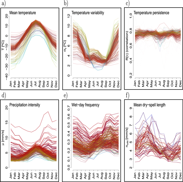
Figure 2. Sensitivity of the observational temperature and precipitation statistics to the mean seasonal cycle: (a) monthly mean temperature, (b)  and (c)
  , (d) wet-day mean precipitation μ, (f) wet-day frequency fw, and (f) the mean number of consecutive dry days ncdd. Each line represent one site and the colour of the curves matches the colour of the location marker in figure 1.
Download figure:
Standard image High-resolution imageA validation of the GCMs was based on a comparison of the standard deviation of the principal components (PCs) from the common EOF analysis over the 1949–2015 interval common to both reanalysis and GCMs. The GCMs simulated spatial patterns of variability for seasonal mean temperatures over the predictor region with similar characteristics as those found in the reanalysis. There were no model that distingushed itself as being consistently poorer or superior to the rest of the ensemble, but the evaluation suggested that different models had different systematic biases (SM). Cross-validation correlation scores and R2 statistics were used to evaluate the step-wise multiple regression used in the ESD, and the results for temperature indicated that the downscaling model could account for about 90% of the seasonal temperature variability. The validation also involved an assessment of the degree that the downscaled ensembles of GCM projections reproduced observed magnitudes of interannual variability and past trends. The trends were in general agreement with observations over common time intervals, and the magnitude of interannual variability was slightly exaggerated by the downscaled ensembles. Overall, the ESD for seasonal mean temperature provided credible results that were consistent with changes in the past.
Projected changes in future temperature and precipitation were based on ESD of entire CMIP5 ensembles and subject to gridding. A 'typical warm winter' in 2099 over Fennoscandia and the high Arctic was estimated to be 7 °C warmer than a corresponding warm winter in 2010 (see SM), given the RCP4.5 emission scenario (figure 3(a)). Generally higher  in the future was a robust feature in all emission scenarios, seasons, and for near, mid, and distant future. These results are presented in the atlas in the SM, showing changes since 2010 in the 95-percentile of the downscaled ensemble. The most extreme warming was associated with emission scenario RCP8.5 and exceeded 18 °C.

Figure 3. Projected change in (a) a typically 'warm' mean winter temperature and the (b) a typically 'wet' warm season μ for 2099, given the emission scenario RCP4.5. Here the typically 'warm' and 'wet' refer to the upper level (95-percentile) of the ensemble spread (one-in-twenty year high value) rather than the ensemble mean, but the upper quantile also represent the results of the climate models with the regional highest climate sensitivity. The maps show the difference between the 95-percentile for 2099 and 2010 respectively.
Download figure:
Standard image High-resolution imageThe evaluation of the ESD method indicated moderate skills for downscaling fw (the occurrence of precipitation) when SLP was used as predictor. The downscaled ensemble results slightly under-estimated the interannual range of variability, and a histogram of past proportional trends in fw exhibited a bimodal structure, which was consistent with increased precipitation frequency in some regions and a decrease elsewhere. One explanation for such regional differences is a shift in the location of storm tracks. The projected changes in fw differed with season, and included regions with both increases and decreases in the range −5–+10% (RCP4.5).
The picture for μ was more complex than for fw, and the evaluation of the ESD method used for projection gave poor skill scores. Nevertheless, the sensitivity analysis suggested a dependency between past trends in μ and  of 8.75% °C−1 which implies an increased winter-time precipitation intensity of 20%–70% by 2099 (RCP4.5), with strongest increase in the region with greatest warming (figure 3(b)). Diagnostics for ESD analysis applied to μ and reanalysis indicated a connection between North Atlantic cyclone activity and intense rainfall along the west coast of northern Norway during both warm and cold seasons. A typical feature in the large-scale temperature over the North Atlantic was a cooler ocean region west off the British Isles and south of Greenland, and higher temperatures further south and over the North Sea. Some of the storm systems from the North Atlantic reach the Barents Sea, and the downscaled results for deep cyclone storm tracks in the Barents region suggested higher frequency in the future and was a robust result with respect to RCP (figure 4).

Figure 4. Projected change in the number of deep synoptic cyclones over the Barents Sea given the emission scenario RCP4.5. The storm statistics were aggregated over the region marked as dashed rectangle in the upper right insert. The observed trend in ns is consistent with those estimated from ESD applied to the RCP4.5 ensemble, and the observed ns falls outside the 90% confidence interval of the ensemble more frequently than a p = 0.1 would imply (see SM).
Download figure:
Standard image High-resolution image
4. Discussion
The results presented here reflected changes in the upper range of the ensembles, taken as the 95-percentile. This upper range was sensitive to both a shift in simulated change in the magnitude interannual variability and the models' different climate sensitivity. There is a complex link between circulation patterns, storm statistics, precipitation and temperature [39] that was emphasised here, and is a small part of a larger information content embedded in large GCM ensembles and historical observations. The use of large ensembles is key, and even if a GCM and an RCM were 'perfect', they would not provide a good picture of weather related risks based on just one simulation because the objective is to predict the longer term statistics for temperature and precipitation.
The lowest confidence of the downscaled results concerned μ and its spatial-temporal intermittency may be one factor explaining its wide range of uncertainty and small effective statistical sample. A small number of very extreme cases can have a strong influence, and the sampling issue is exacerbated by the rain gauges' small cross-section area of capture. In addition, a number of different phenomena are known to produce precipitation such as cyclones, fronts, orographic effects and local cumulonimbus, and precipitation has geographically distributed sources of moisture. The downscaling in this study was designed to capture precipitation connected with storms and remote moisture sources, but not local cumulonimbus and the effect of increased area of open ocean on μ [40, 41]. Nevertheless, there were multiple indications suggesting that a higher temperature is associated with an increase in μ, and these effects can to some degree be accounted for in terms of the ratio of local trends in μ and  respectively. The dependency between these local trends was considered to be more reliable than the results from ESD based on North Atlantic temperatures, due to the poor ESD skill scores.
Another caveat was that the recorded increase in the precipitation may be due to a changing portion of the precipitation falling as snow and rain and systematic under-catch of snow [42]. Evaporation E takes place over a wide area AE but the precipitation P involves a more limited area AP (cloud-covered area where  ). A constant atmospheric water vapour content implies that the global rate of evaporation equals the global rate of precipitation averaged over time and space:
  . Since these involve different areas, an increase in the precipitation is expected to be proportionally higher than the evaporation by a factor of γ, as in
  , where
  and
and  is the spatial average. In other words, we can deduce that the precipitation will increase faster than the atmospheric moisture because E is a smooth variable in space but P is intermittent in time and space.
Another caveat concerns the variable station network density, and there were fewer data points in Russia which emphasises Fennoscandia with a dense network (figure 1). This choice influenced the selection of predictor domain and the ESD in terms of favouring the heavy precipitation over northern Norway and its association with low-pressure systems. A sparse Russian network of stations also has an effect of the gridding of the results.
The present study was limited to a small set of climate parameters and there is a need for future work addressing the question of downscaling precipitation and additional statistics, such as the number of days with above- or below-freezing temperatures, the length of the winter season, and the future prospect for the snow cover. Such analyses may make use of dependencies between the seasonal mean temperature and number of warm/cold days for some sample stations [14], in addition to probabilities of heavy precipitation associated with μ and fw [25, 26]. There is also a risk for abrupt changes and a triggering of tipping points, which may or may not be captured by GCMs, e.g. a collapse of ice sheets, release of methane, and rapid changes to the landscape and vegetation. Nevertheless, the projections presented here show the best current information there is on future climate outcomes in the Arctic.
5. Conclusions
Projected changes in climate parameters for the Barents region indicate a temperature increase for 'typical warm' winters with ∼7 °C over northern Fennoscandia by 2099 and the high Arctic under the RCP4.5 emission scenario. The scenarios for the wet-day frequency and mean precipitation were not as robust with respect to greenhouse gas emissions and season as for temperature, however, the inferred changes in the wet-day mean were most severe in winter (up to 70% for 2099 and RCP4.5). The wet-day frequency pointed to greatest increases ( 5%–10%) along the northern coast of Norway but reduced frequencies in northern Sweden and the vicinity of the Bothnian Bay. The number of deep synoptic cyclones can also be expected to increase in a warmer Arctic, but there was little indication that persistence in the temperature and precipitation will change in the future.
Acknowledgments
This work was supported by the Norwegian Meteorological Institute, and carried out for AMAP/AACA. We acknowledge the efforts by the IMILAST team for the cyclone analysis, ECA&D for the station data, the team behind the NCEP/NCAR reanalysis, and the people behind the CMIP5 results.