

Abstract
Artificial ocean alkalinization (AOA) is investigated as a method to mitigate local ocean acidification and protect tropical coral ecosystems during a 21st century high CO2 emission scenario. Employing an Earth system model of intermediate complexity, our implementation of AOA in the Great Barrier Reef, Caribbean Sea and South China Sea regions, shows that alkalinization has the potential to counteract expected 21st century local acidification in regard to both oceanic surface aragonite saturation Ω and surface pCO2. Beyond preventing local acidification, regional AOA, however, results in locally elevated aragonite oversaturation and pCO2 decline. A notable consequence of stopping regional AOA is a rapid shift back to the acidified conditions of the target regions. We conclude that AOA may be a method that could help to keep regional coral ecosystems within saturation states and pCO2 values close to present-day values even in a high-emission scenario and thereby might 'buy some time' against the ocean acidification threat, even though regional AOA does not significantly mitigate the warming threat.
Export citation and abstract BibTeX RIS

Original content from this work may be used under the terms of the Creative Commons Attribution 3.0 licence. Any further distribution of this work must maintain attribution to the author(s) and the title of the work, journal citation and DOI.
1. Introduction
Anthropogenic CO2 invades the ocean and thereby perturbs ocean chemistry, this phenomenon is also known as 'ocean acidification' (e.g. Caldeira and Wickett 2003, Feely et al 2004). If CO2 emissions continue to increase and the ocean continues to become more acidic these changes will further affect the ambient saturation state of aragonite (described by aragonite Ω). Since calcification, which is a crucial skeleton building process for most stony corals, is considered to be highly sensitive to ambient aragonite Ω, coral calcification is likely to become inhibited in the future (Gattuso et al 1998, Langdon and Atkinson 2005). Stony coral reefs sustain the most diverse ecosystems in the tropical oceans, and the coral-supported tropical fish (Munday et al 2014), coralline algae (Mccoy and Ragazzola 2014), echinoderms (Dupont et al 2010), molluscs (Gazeau et al 2007), crustaceans (Whiteley 2011), and corals themselves (Kleypas et al 1999a, Hoegh-Guldberg et al 2007, Cao and Caldeira 2008, Crook et al 2011, Meissner et al 2012a) are expected to face difficulties in adapting to future ocean conditions in coming decades because of both ocean acidification itself and the loss of the reef structure. A potential loss of coral reefs and their ecosystems may also have a direct impact on coastal resources and services (Brander et al 2012). Besides the threat from ocean acidification coral reefs face a number of other significant threats such as coral bleaching, which is triggered by persistent heat stress and is thought to be one of the most serious climate change related threats (Hoegh-Guldberg 1999, Cooper et al 2008, De'ath et al 2012, Frieler et al 2012, Caldeira 2013).
Since efforts to mitigate global warming and ocean acidification by reducing emissions have, up to now, been unsuccessful in terms of a significant reduction in the growth of atmospheric CO2 concentrations, there has been growing interest in climate engineering (CE) to mitigate or prevent various consequences of anthropogenic climate change (Crutzen 2006, Schuiling and Krijgsman 2006, Oschlies et al 2010). For example, several modeling studies have examined 'artificial ocean alkalinization (AOA)' which modifies ocean alkalinity. These studies simulated the use of alkalizing agents such as olivine (a Mg–Fe–SiO4 mineral) (Köhler et al 2010, 2013, Hartmann et al 2013), calcium carbonate (Caldeira and Rau 2000, Harvey 2008), or calcium hydroxide (Ilyina et al 2013a, Keller et al 2014) to elevate the ocean's alkalinity to increase CO2 uptake and mitigate ocean acidification. While these simulations suggested that AOA could potentially be used to mitigate global warming and ocean acidification to some degree, some studies also suggested that deploying AOA at a global scale may face prohibitive logistical and economical constraints and could possibly cause undesired side effects (Renforth et al 2013, Keller et al 2014).
In this paper we use Earth system model simulations of regional AOA to investigate the potential of AOA to protect specific stony coral reef regions against ocean acidification. We also investigate possible environmental side effects of AOA and possible regional differences in effectiveness or undesired side effects. The model simulations show AOA could mitigate ocean acidification in our investigated coral reef regions, albeit at substantial economic costs and with the termination risk of a rapid return to acidified conditions after the stop of local AOA.
2. Methods
We simulated calcium hydroxide (Ca(OH)2) based AOA in the Great Barrier Reef (GB, 9.0° S–27.0° S, 140.4° E–154.8° E, an area of 1.7 × 10⁶ km2), the Caribbean Sea (CS, 10.8° N–27° N, 68.4 °W–93.6° W, an area of 3.9 × 10⁶ km2) and the South China Sea (SC, 0° N–23.4° N, 104.4° E–129.6° E, an area of 5.2 × 10⁶ km2) (figure 1) using the University of Victoria Earth System Climate Model (UVic) version 2.9. These areas contain some of the world's most abundant coral reefs (http://reefbase.org/) and are large enough to be addressed by the UVic model. From the data obtained from ReefBase (http://reefbase.org/), we found that from a total of 10 048 coral reef locations, 3323 are located in the Great Barrier Reef box, 601 in the Caribbean Sea box, and 2060 in the South China Sea box. Altogether 5984 reef points are included in our three regions, which is more than half of the global coral reef locations collected from ReefBase.

Figure 1. Annual mean surface aragonite Ω and pCO2 simulated by the UVic model control run without regional artificial ocean alkalinization (AOA) for preindustrial (a), (c) and 2020 (b), (d). AOA experimental regions are marked by black boxes. Coral Reef locations are marked in cyan.
Download figure:
Standard image High-resolution imageThe UVic model consists of an energy-moisture balance atmospheric component, a 3D primitive-equation oceanic component that includes a sea-ice sub-component, and a terrestrial component (Weaver et al 2001, Meissner et al 2003). Wind velocities are prescribed from National Center for Atmospheric Research (NCAR)/National Centers for Environmental Prediction (NCEP) monthly climatological data. Accordingly, UVic does not feature decadal ocean–atmosphere oscillations, like El Niño-Southern Oscillation (ENSO). The model has a spatial resolution of 3.6° × 1.8° with 19 vertical layers in the ocean. The global carbon cycle is simulated with air–sea gas exchange of CO2 and marine inorganic carbonate chemistry following the Ocean Carbon-Cycle Model Intercomparison Project Protocols (Orr et al 1999). The inorganic carbon cycle is coupled to a marine ecosystem model that includes phytoplankton, zooplankton, detritus, the nutrients nitrate and phosphate, and oxygen (Keller et al 2012). The model has been evaluated in several model intercomparison projects (Weaver et al 2012, Eby et al 2013, Zickfeld et al 2013), and shows a reasonable response to anthropogenic CO2 forcing that is well within the range of other models. In order to illustrate that our model is robust in reproducing general ocean circulation and chemistry, we validate our model against Global Ocean Data Analysis Data Project (GLODAP) v1.1 data for ocean total alkalinity and oceanic dissolved inorganic carbon (Key et al 2004) (figures S1 and S2 in supplementary materials), Surface Ocean CO2 Atlas (SOCAT) data (Bakker et al 2014, Landschützer et al 2014) for sea surface pCO2 (figure S3), and World Ocean Atlas (WOA) 2013 data for sea surface temperature (SST) (figure S4). The validation illustrates that UVic can generally reproduce the global patterns of surface ocean alkalinity and dissolved inorganic carbon as well as sea surface pCO2. UVic's performance in reconstructing SST is also generally good, especially in regions where AOA is implemented in our study with less than a 0.8 °C model-data misfit. Overall, the model-data differences displayed by the UVic model are well within the range of data-error from the 5th Coupled Model Intercomparison Project (CMIP5) model simulations (Jungclaus et al 2013, Ilyina et al 2013b, Wang et al 2014).
The model was spun-up for 10 000 years under pre-industrial atmospheric and astronomical boundary conditions. From year 1800 to 2005 the model was forced with historical fossil fuel and land-use carbon emissions. Then, from the year 2006 onwards the Representative Carbon Pathway 8.5 (RCP 8.5) anthropogenic CO2 emission scenario forcing was used (Meinshausen et al 2011). CO2 is the only greenhouse gas taken into account. Continental ice sheets, volcanic forcing, and astronomical boundary conditions were held constant to facilitate the experimental set-up and analysis.
Ca(OH)2 based AOA is simulated in an idealized manner by increasing surface alkalinity (Keller et al 2014). The rationale behind this method is that dissolving one mole of Ca(OH)2 in seawater increases total alkalinity by 2 moles (Ilyina et al 2013a). We simulate Ca(OH)2-based AOA by homogeneously and continuously adding alkalinity to the upper 50 m of the targeted regions. In the following, we therefore use the term 'lime addition' to refer to our simulated Ca(OH)2 addition. Directly simulating individual reefs or corals is beyond our current model's capacity and we therefore focus on AOA-induced impacts on regional and global marine chemistry. Also, we ignore the impact of increasing water temperature on corals, which will accompany elevated levels of atmospheric CO2 and would likely also have a detrimental impact on coral reefs.
We use a fixed threshold aragonite Ω to describe suitable stony coral habitats since most of today's coral reefs are found in waters with ambient seawater aragonite Ω above a critical value (Kleypas et al 1999b, Meissner et al 2012a, 2012b, Ricke et al 2013). However, this approach involves some uncertainties (Kleypas et al 1999b, Guinotte et al 2003) due to the neglect of seasonal and diurnal Ω fluctuations, species variety, and species ability to adapt. Critical coral habitat threshold values of ambient aragonite Ω ranging from Ω = 3 (Meissner et al 2012b), Ω = 3.3 (Meissner et al 2012a), to Ω = 3.5 (Ricke et al 2013) have been used in recent climate change studies, acknowledging that these represent regional mean values and that local reef-scale carbonate chemistry may display large diurnal fluctuations also in healthy reefs. Ignoring SST as a regulator of coral reef habitats may be a further simplification (Couce et al 2013).We follow these earlier studies and, in this paper, use an aragonite Ω threshold of 3 to determine whether or not seawater chemistry with a region is suitable for stony corals.
A healthy coral ecosystem usually includes a multitude of both calcifying and non-calcifying organisms. Aragonite Ω is commonly used to evaluate the impact of ocean acidification on marine calcifying organisms. Nevertheless, ocean acidification can also affect non-calcifying organisms, e.g. by reducing their metabolic rates (Rosa and Seibel 2008) or damaging their larval and juvenile stages (Frommel et al 2011). Concerning non-calcifying organisms, often pCO2 is employed as a metric to evaluate impacts of ocean acidification. We therefore also consider how seawater pCO2 will develop under increasing atmospheric pCO2 and continuous AOA. Without AOA, annual mean surface seawater pCO2 will follow atmospheric pCO2 with some small time lag (e.g. Bates 2007). A meta-study of resistance of different marine taxa to elevated pCO2 (Wittmann and Pörtner 2013) found that 50% of the species of corals, echinoderms, molluscs, fishes and crustaceans are negatively affected if seawater pCO2 reaches high levels (between 632 and 1003 μatm) with many species, except for crustaceans, also being significantly affected by pCO2 levels between 500 and 650 μatm. Among the studied species, 57% of echinoderms and 50% of molluscs were negatively affected by the lowest levels of experimental pCO2 manipulations. Since the loss of even one species, such as a keystone species, could potentially be detrimental for reef health, we chose a relatively low threshold of 500 μatm pCO2 (as an annual average) to determine whether or not conditions were suitable for maintaining a healthy reef habitat. Moreover, by choosing a lower threshold we can better account for any variability in pCO2 that may not be well simulated by our model. However, we must acknowledge that there are considerable uncertainties concerning such a threshold. Furthermore, these thresholds can be modulated by other environmental factors (Manzello 2015) and may not be absolutely applicable in every reef location. To avoid unnecessary complexity, the thresholds for both pCO2 and Ω are considered here in terms of regional and annual averages.
Four sets of model simulations were carried out (table 1), beginning at the start of the year 2020 and ending at the end of the year 2099 of the RCP 8.5 emission scenario. Ensemble A is the control run (no AOA). In Ensemble B constant amounts of lime (from 1 to 10 Gt yr−1 with 1 Gt yr−1 increments) were added homogenously to each region. In Ensemble C we sought a solution where a linear increase of AOA over time ensured that our thresholds were met with a minimum lime addition, with the chosen rate of increase guided by the results from Ensemble B. Runs of Ensemble D are identical to those of Ensemble C, except for the fact that we stop AOA at the beginning of the year 2070 and continue the run without AOA until the end of the year 2099. This is to study the impact of a planned or unplanned stop of AOA.
Table 1. Description of simulated artificial ocean alkalinization (AOA) experiments during RCP 8.5 CO2 emissions scenario forcing.
| Experimental ensemble | AOA starts in year | AOA ends in year | Lime addition (Gt yr−1) | Number of runsa |
|---|---|---|---|---|
| A (control) | — | — | 0 | 1 |
| B (constant addition) | 2020 | 2099 | 1, 2, 3, 4, 5, 6, 7, 8, 9, and 10 | 10 |
| C (optimal) | 2050b or 2048c | 2099 | Linear increase with time | 60 |
| D (optimal/termination) | 2050b or 2048c | 2070 | Linear increase with time | 60 |
aIn each region respectively. bGreat Barrier Reef. cCaribbean Sea and South China Sea.
3. Results
In the control run, regionally averaged surface aragonite Ω drops below 3 in the Great Barrier Reef (GB) after year 2057, in the Caribbean Sea (CS) after year 2049, and in the South China Sea (SC) after year 2057 (figure 2). The mean pCO2 threshold of 500 μatm is crossed in the GB at year 2050, in the CS at year 2048, and in the SC at year 2048. With constant AOA (Ensemble B) the thresholds are crossed at a later date or not at all, depending on the intensity of AOA. After an initial increase of Ω and decrease of pCO2, respectively, the surface aragonite Ω declines and pCO2 increases almost linearly with time as ocean acidification intensifies because of the increasing invasion of atmospheric CO2. The minimum amount of lime that is needed to prevent regionally averaged surface aragonite Ω from dropping below 3 before the end of year 2099 in these constant AOA simulations is 1.1 (GB), 1.9 (CS), and 1.5 Gt yr−1 (SC), respectively. In order to prevent regional annual-mean surface pCO2 from exceeding 500 μatm, the minimum amount of lime that is needed is always significantly larger, i.e. 2.5 (GB), 4.9 (CS), and 5.7 Gt yr−1 (SC), respectively. These results indicate that meeting the pCO2 threshold in our setup always requires a higher alkalinity addition than it does to meet the aragonite saturation threshold, thus in our particular case of combined pCO2 and Ω thresholds, only the pCO2 threshold needs to be considered.
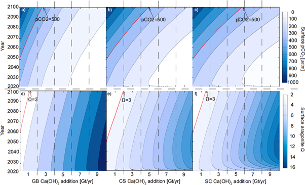
Figure 2. Regionally-averaged surface aragonite Ω and surface pCO2 that occur in the Great Barrier Reef (a), (d), Caribbean Sea (b), (e), and the South China Sea (c), (f) regions for the Ensemble A and B simulations as a function of time. Thresholds are highlighted by red isoclines.
Download figure:
Standard image High-resolution imageEnsemble C includes a total of 60 model runs for each region that were initiated with output from the control run years 2050 (GB) and 2048 (CS and SC), respectively, which are the time points just before our chosen threshold values for surface pCO2 was crossed in the respective experimental regions. Thereafter, simulated lime additions increase linearly from 0 Gt yr−1 to a maximum addition in year 2099, which ranges from 2 to 7 Gt yr−1 depending on the region (not shown; see figure 3(d) for the 'optimal' example). Of the 3 × 60 runs composing Ensemble C, our specific interest was in the runs ending at 2.7 (GB), 5.1 (CS) and 6.1 (SC) Gt lime per year (year 2100) since these 'optimal' runs require the least time integrated amount of AOA to prevent our chosen thresholds from being crossed (figure 3(b)). In year 2099 of these runs we find surface aragonite Ω = 4.3, 4.6, and 5.7 and surface pH = 7.99, 8.03, and 8.04 in the GB, CS, and SC, respectively (figure 3(a)). That is, in order to prevent local seawater pCO2 from increasing above our chosen threshold, one would have to accept a considerable increase in seawater Ω compared to the situation in 2020. In the year 2099, the region-averaged alkalinity additions are 42.6 mol m−2 yr−1 (GB), 34.9 mol m−2 yr−1 (CS) and 31.2 m−2 yr−1 (SC). This regional AOA leads to an additional global oceanic carbon uptake of ∼15.36, 32.54, and 35.41 Gt C for the GB, CS, and SC runs by the end of the year 2099, respectively.

Figure 3. Comparison between the Great Barrier Reef, Caribbean Sea, and South China Sea regionally averaged annual surface aragonite Ω (a), seawater pCO2 (b), and sea surface pH (c) values during the control (Ensemble A) and the 'optimal' AOA simulations (single optimized simulation from Ensembles C and D). Note that AOA ends in the year 2070 in the Ensemble D simulations. The amount of lime needed for the 'optimal' AOA implementation in year 2100 is labeled in (d).
Download figure:
Standard image High-resolution imageTerminating regional AOA (Ensemble D) has a strong and rapid impact on surface aragonite Ω, seawater pCO2 and pH in the respective regions (figure 3). After termination the AOA related regional changes disappear on an annual timescale and quickly converge back to conditions very close to those of the control run.
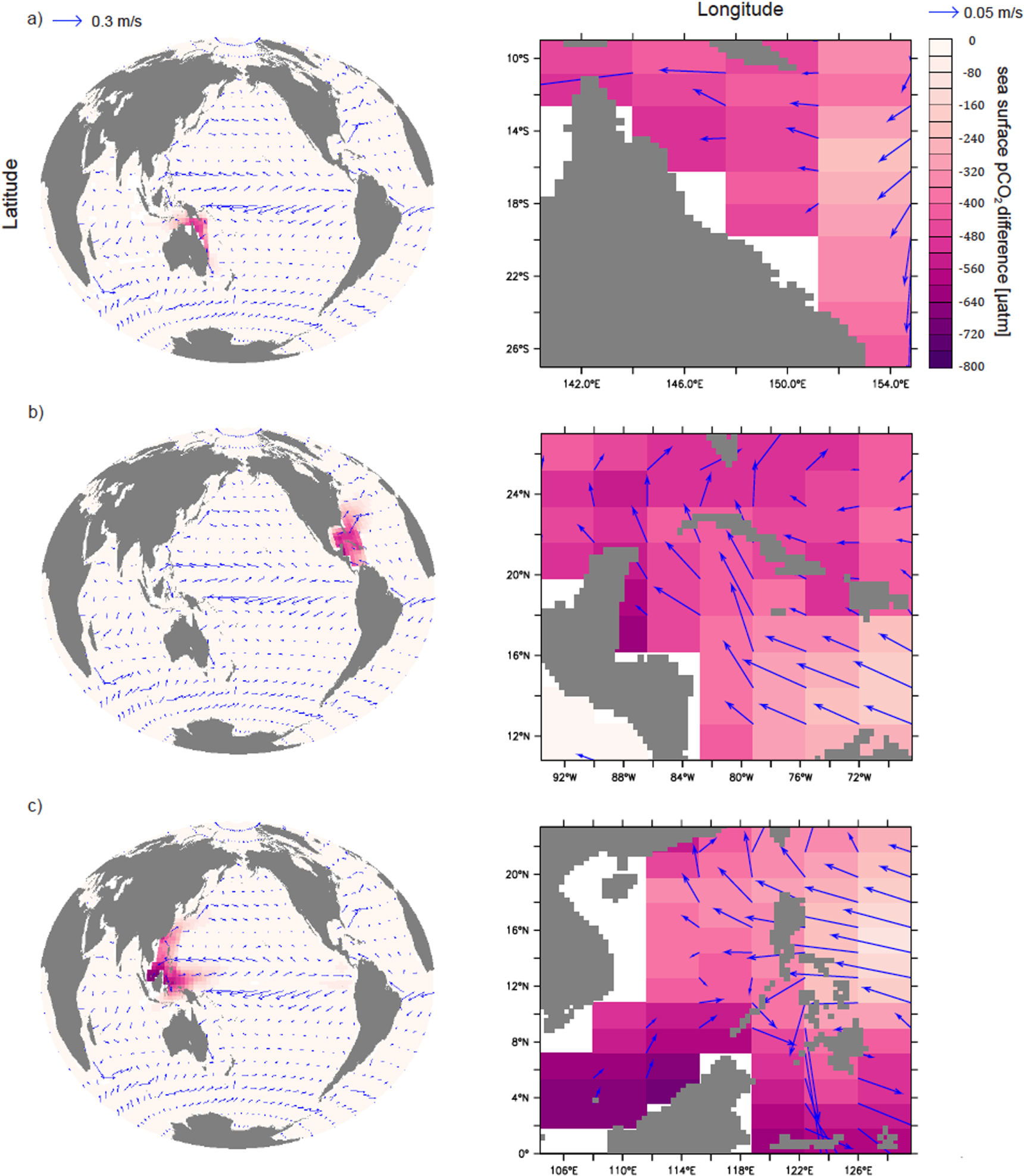
Regional AOA also has effects on global ocean biogeochemistry (figures 4 and 5). Within a few decades, AOA in the CS affects surface Ω and seawater pCO2 in much of the western North Atlantic. On the timescales considered, AOA in the GB region appears to be the most locally confined in our runs, but nevertheless affects the coastal waters of Papua New Guinea and Indonesia. Overall, however, remote effects are moderate compared with local impacts. Compared with the control run, the optimal runs (Ensemble C) have annual regional surface pCO2 partial pressures that are ∼300–800 μatm lower and an aragonite Ω that is of ∼2.5–10 times higher in AOA regions compared to the control run without AOA. At the same time, both the globally averaged increase in surface Ω and the decrease in pCO2 are moderately small (figure S5 in supplemental materials). Thus, in our optimal AOA simulations, atmospheric CO2 is drawn down by the end of 2099, relative to the control run, by about 7 ppm for GB run, 15 ppm for CS run and 16 ppm for SC.
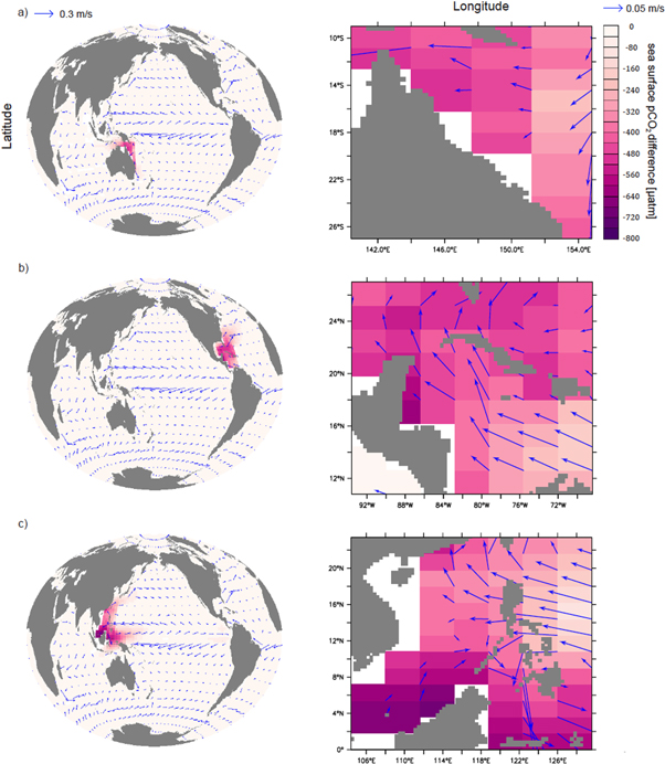
Figure 4. Simulated year 2099 surface pCO2 differences between the optimal runs (Ensemble C) and the control run for the Great Barrier Reef (a), Caribbean Sea (b), and South China Sea (c). Each is shown with respect to the global impact (left) and the impact over the respective region where AOA is applied (right). Annual mean surface current velocities are marked as blue arrows.
Download figure:
Standard image High-resolution image
Figure 5. Simulated year 2099 surface aragonite Ω differences between the optimal runs (Ensemble C) and the control run for the Great Barrier Reef (a), Caribbean Sea (b), and South China Sea (c). Each is shown with respect to the global impact (left) and the impact over the respective region where AOA is applied (right). Annual mean surface current velocities are marked as blue arrows.
Download figure:
Standard image High-resolution image
4. Discussion
From a marine biogeochemical perspective, our results indicate that regional AOA could potentially be an effective means to mitigate regional ocean acidification. In our AOA simulations (Ensemble B, C and D) the increase of surface seawater pCO2 levels, as well as the reduction of local pH and aragonite saturation states are all mitigated or even reversed in the targeted regions (figures 2– 4). However, increasing surface ocean alkalinity also induces an additional uptake of CO2. For the optimal runs (Ensemble C), AOA modifies the oceanic DIC system (figure S6) leading to an increase in both carbonate and bicarbonate ions. The increase of Ω and the carbonate ion concentration beyond current or preindustrial levels in figure 3(a) may have unforeseen consequences in the real ocean as elevated supersaturation may have biological impacts (Cripps et al 2013) or even cause the spontaneous abiotic precipitation of CaCO3. Like the biotically induced precipitation of CaCO3, this process would directly lead to an increase of pCO2, i.e. constituting a negative feedback to intentional alkalinization. If spontaneous CaCO3 precipitation due to elevated total alkalinity happens, this would be detrimental as coral reefs are known to be sensitive to high levels of turbidity (Broecker and Takahashi 1966, Roy and Smith 1971). Previous research by Renforth et al (2013) suggest to use an optimum lime particle size of 80–100 since such particles can be fully dissolved in a typical surface ocean with a depth less than 100 m. For most tropical stony coral ecosystems, which are generally within 100 m of the surface, the direct addition of such particulate lime could affect water column transparency and may even result in particles settling directly onto organisms. To minimize this side effect, lime could be dissolved in seawater before adding it.
In addition to CO2-system changes, AOA, if done with lime, will add calcium to the system. In our optimum simulations (Ensemble C), the surface calcium concentration could be elevated by up to 0.16, 0.26, and 0.34 mmol kg−1 for the GB, CS, and SC respectively (figure S7 in supplementary materials). Natural calcium behaves conservatively in the ocean and for a salinity of 35 the calcium concentration is about 10.27 mmol kg−1 (Pilson 2013). The amount of calcium added during alkalinization is hence less than 4% of the background calcium concentration.
How well do our simulations reflect the real environmental conditions that coral reef ecosystems might experience during a high CO2 climate scenario (control run) and AOA deployment? An estimate of potential impacts of model errors in simulated carbonate chemistry (table S1) suggests uncertainties in the calculated regionally averaged alkalinity requirements of less than 10%. This result indicates that the seawater chemistry simulated by UVic is acceptable for such an initial study of potential AOA. Three limitations of our study, however, remain: first, the current model's coarse resolution does not resolve small-scale physical processes like boundary currents, local upwelling and temperature variability around reef archipelagos or in shallow lagoons (Meissner et al 2012a). Studies with higher resolution models would be necessary to assess these local aspects. Second, most reported massive coral bleaching incidents are associated with El-Niño years (Aronson et al 2002), which are not resolved in our UVic model simulations driven by climatological winds. The observed ENSO-associated variability in our studied regions is relatively weak, as revealed by an analysis of historical SST and air–sea delta-pCO2 records (supplementary figures S14 and S15). However, it is not well known how ENSO variability will develop in the future (Guilyardi et al 2009, Collins et al 2010) and thus its impact on our study region will remain another uncertainty. Third, local calcification, dissolution, photosynthesis and respiration within coral reefs affect local ocean chemistry and are not in detail included in our model. For example, over a diel cycle the aragonite saturation state may vary considerably, as has been observed at a coral reef off Okinawa, Japan where Ω ranged from 1.08 to 7.77 (Ohde and Hossain 2004). Similarly, seawater pCO2 has been observed to vary between 420 and 596 μatm during a 24 h period (Dufault et al 2012). These large variations are due to day-night fluctuations in carbon uptake and metabolism within coral reefs (Comeau et al 2012), which our model cannot simulate. Because the ocean's uptake of anthropogenic CO2 is associated with a decrease in the ocean's buffering capacity, natural fluctuations of the carbonate system on seasonal and diurnal scales are expected to increase (Riebesell et al 2009, Melzner et al 2012). Lacking the small-scale variability in general, our simulations may underestimate the stress that might go along with even stronger fluctuations in the future. However, since AOA would increase the regional ocean buffering capacity, it could dampen future carbonate system fluctuations otherwise expected in a high CO2 emission world.
Our results also reveal different regional sensitivities of the AOA deployments. To stay within our chosen mitigation guardrails (seawater pCO2 < 500 μatm, Ω > 3 in the regional and annual means) during the 21st century the GB requires the smallest amount of total lime input while the SC requires the largest. These differences are largely due to the size difference of our studied regions. In the year 2099, the regional mean alkalinity additions are 42.6 mol m−2 yr−1 (GB), 34.9 mol m−2 yr−1 (CS) and 31.2 molm−2 yr−1 (SC). These differences can be explained by a combination of local hydrography and biogeochemistry. For example, the local surface alkalinity decline during the first year after AOA termination in Ensemble D, i.e. between the beginning and end of year 2070 is largest in CS (80 mmol m−3), intermediate for GB (70 mmol m−3) and smallest for SC (61 mmol m−3). Figure 3(b) reveals that even though surface pCO2 is almost identical in the three areas, the evolution of surface aragonite saturation levels during AOA differs among the regions (figure 3(a)). For the same pCO2 levels, aragonite Ω in the SC increases more rapidly than in the CS and GB. This variation in carbonate chemistry also leads to regionally different sensitivities to ocean acidification, which determines the initiation and duration of AOA in Ensemble C.
The effectiveness of AOA can be described by the ratio between oceanic inventory changes of DIC referenced to the control run and added total lime by the end of year 2099. The optimal runs of Ensemble C show an effectiveness of 1.4 for GB, 1.5 for CS and 1.4 for SC, close to the value of 1.4 that we calculated based on data from Keller et al (2014). Compared to previous estimates of AOA effectiveness that are above 1.6 (Renforth et al 2013), our slightly lower values can be explained by the downward transport of added alkalinity on time scales shorter than the air–sea equilibration time of CO2 (figure S8 in supplementary material). This loss of alkalinity from the surface layer leads, in our model, to a lower effectiveness than predicted by theory and adds another element of uncertainty to predicting how AOA would work if actually deployed.
General surface ocean acidification can be detected in the runs of ensemble C until the year when AOA is initiated (figure S9 in supplementary material). Thereafter total alkalinity accumulates until year 2099 with regional TA reaching concentrations about 200–500 mmol m−3 higher than the initial values. Comparisons between this study and other AOA studies that included regional applications, such as Ilyina et al (2013a), are difficult because those studies were designed to investigate AOA as a means for global CO2 mitigation, and thus even when AOA was applied regionally it was in still relatively large areas that have a high potential for increasing the uptake of atmospheric CO2. An implementation of AOA on a regional scale of less than 10 geographical degrees across for only a short time of less than 100 years, has only a limited impact on atmospheric CO2, while a global implementation of AOA (Keller et al 2014), in particular when applied for centuries to millennia (Ilyina et al 2013a), can significantly impact atmospheric CO2 and the global carbon cycle. In contrast to results of the global AOA studies, only a relatively low carbon sequestration and storage potential, with less than a 20 ppm atmospheric CO2 reduction, is achieved in our regional AOA simulations. In Keller et al (2014) a global implementation of lime-based AOA is deployed from year 2020 to year 2100 leads to an atmospheric CO2 decrease about 166 ppm, while Ilyina et al (2013a) observe a CO2 drawdown of up to 450 ppm in their global and 'Atlantic+Pacific' AOA implementation scenarios. Our results imply that from the regions we selected, regional and decadal- to centennial-scale AOA would not be an appropriate means for significant climate remediation.
Differences between regional and global AOA also affect the local seawater chemistry after a termination of AOA. If regional AOA is terminated abruptly, regional seawater pCO2, aragonite Ω and pH rapidly return to the levels found in the control run (figure 3) on an annual timescale. This is different from the findings of large-scale AOA simulations where such a termination effect is not observed (Ilyina et al 2013a, Keller et al 2014). In the case of regional AOA, lime and the dissolution products are dispersed rapidly and diluted by seawater from outside the deployment area. Such a rapid change in regional ocean chemistry, which is faster than in any climate change scenario, could potentially put substantial stress on regional ecosystems. Thus, if regional AOA was done without reducing atmospheric CO2, the process of adding lime would potentially have to continue for very long times or be phased out carefully to avoid risks to coral reef ecosystems.
A practical consideration is how much our optimal AOA applications would cost. For CaO-based AOA (Ca(OH)2 is hydrated CaO) cost estimates provided by Renforth et al (2013) indicate that every ton of CO2 taken up by the ocean as a result of AOA costs approximately $72–159 (US dollars). These estimates include the extraction, calcination, hydration, and surface ocean dispersion costs associated with AOA and are likely higher than AOA in our study would be since the transportation costs were based on covering the entire global ocean. In our optimal simulation, the cumulative amount of atmospheric CO2 that is sequestered by AOA in the year 2099 is 56.32 Gt CO2 in the GB, 119.28 Gt CO2 in the CS and 129.84 Gt CO2 in the SC. Based on Renforth et al (2013), AOA would cost around US$ 51–112 billion for the GB per year (if we assume an even sharing of costs over the 80 year periods of our AOA simulations), US$ 107–237 billion for the CS per year, and US$ 117–258 billion for the SC per year. Among all three studied regions, GB has the largest number of coral reef locations and the AOA costs for it are the lowest from our study. The Gross Domestic Product (GDP) for Australia in the year 2014 was US$ 1.45 trillion. According to our model results, Australia could keep the GB region from crossing our chosen guardrails by spending 3.5%–7.7% of its GDP for coral reef protection. Admittedly, this is a huge investment compared with the estimated benefits (5–7 billion US$ per year) related to coral reefs (GBRMPA 2013).
Ocean acidification is only one of the stressors that corals reefs face in the future. Our study has not addressed other problems such as overfishing (Loh et al 2015) or thermal stress (Goreau and Hayes 1994). Coral reef bleaching, caused by thermal stress, is one of the most lethal and enduring threats to coral reefs. For example, in the Great Barrier Reef, between 11% and 83% of coral colonies were affected by large-scale bleaching due to unusually high temperatures during 1998, an El-Niño year, with the mortality rate varying between 1% and 16% (Marshall and Baird 2000). The GB coral coverage declined by around 50% between 1985 to 2012, with 10% of the total loss attributed to coral bleaching (De'ath et al 2012). In the Caribbean Sea (CS), thermal stress in the year 2005 exceeded observed levels in the previous 20 years causing over 80% of corals to bleach and resulting in a 40% population loss (Eakin et al 2010). In the South China Sea (SC), massive coral bleaching in 1997 and 1998 affected 40% of coral colonies, but many of them recovered within a year (Waheed et al 2015). Model simulations have suggested that coral bleaching incidents will increase with global warming, and the threat will become more severe in the future if CO2 emissions remain high and significant warming occurs (Frieler et al 2012, Caldeira 2013). According to Teneva et al (2012)'s model simulations, our three study areas are in coral bleaching hot spots (Goreau and Hayes 1994) with a middle to high likelihood of experiencing bleaching. Donner (2009) predicted that the 10 years' mean SST during 2090–2099 in our studied regions are 3.2 °C (SC), 3.3 °C (GB) and 3.4 °C (CS) higher than those during 1980–2000 under a business-as-usual high CO2 emission scenario. Given such predictions, the question arises as to whether or not regional AOA would be sufficient if CO2 emissions remain high, e.g., warming might harm coral reefs long before acidification becomes a significant threat. There have been proposals to use cloud brightening (Latham et al 2013) to cool down surface temperatures to prevent coral bleaching and it is possible that other solar radiation management (SRM) methods may be envisaged in a similar manner. If SRM were seriously considered for this purpose when atmospheric CO2 levels are high, AOA would be worth considering as well.
5. Conclusions
Our results show that with simulated AOA, regional surface aragonite Ω and pCO2 could be prevented from crossing the acidification thresholds that we set (pCO2 < 500 μatm, Ω > 3). In this respect, marine biota could benefit from AOA. To successfully protect corals and associated marine biota from OA within all three regions examined in our study, one would need to deploy about 356 Gt lime over next 80 years, with estimated implementation costs between 275 and 607 billion US dollars annually. This can possibly 'buy some time' before ocean acidification induces physiological stress and ecological shifts. We have also shown that the carbon sequestration potential of regional AOA is small, with regional differences in its effectiveness and sensitivities. Due to rapid exchange with untreated waters from outside the regions, a termination effect would have to be taken into account should deployment of regional AOA be considered in reality. This research shows that AOA has the potential to mitigate regional ocean acidification for the purpose of protecting tropical coral reef ecosystems. Details about environmental side effects will have to be explored with higher resolution models and dedicated lab and possibly field experiments. From a climate change perspective the best solution would obviously be to stop emitting CO2 and thereby prevent warming and ocean acidification from occurring and affecting coral reef ecosystems in the first place. Since this is unlikely to happen in the near future, it is worth investigating CE methods such as AOA, since they might be able to provide an alternative or complementary means of protection.
Acknowledgments
This is a contribution to the SPP 1689 'Climate Engineering—risks, challenges, opportunities?' funded by the Deutsche Forschungsgemeinschaft (DFG). Additional funding was provided by the BMBF BIOACID Program (FKZ 03F0608A) to WK. All authors declare that they have no potential conflicts of interests.