

Abstract
The dispersion of surface drifters released over a 7-year period from five locations in the southern Gulf of Mexico is described. It is shown that the drifter dispersion is strongly affected by the main mesoscale circulations features frequently observed in this area. Some of them are the anticyclonic eddies shed by the Loop Current at the eastern side of the Gulf of Mexico, and a semi-permanent cyclonic gyre at the Bay of Campeche. The results are examined further in terms of two dominant and contrasting dispersion scenarios: (i) an intense northward advection of drifters, preferentially along the western margin, and (ii) the retention of drifters in the southernmost part of the Gulf of Mexico. The results are discussed from an environmental point of view, by considering particle dispersion from point sources as an approach to study marine pollution problems.

Original content from this work may be used under the terms of the Creative Commons Attribution 3.0 licence. Any further distribution of this work must maintain attribution to the author(s) and the title of the work, journal citation and DOI.
1. Introduction
The Gulf of Mexico (hereafter referred to as GM) is a semi-enclosed sea that belongs to Mexico, the USA and Cuba, where numerous commercial and industrial activities take place in both shallow and deep water regions. Some of the most important are related with oil and gas exploration and extraction by the USA along the northern margins, and by Mexico at western and southern areas. Thus, the study of dispersion phenomena is highly relevant to analyze potential problems of marine pollution in the region.
In this letter we address the problem of surface particle dispersion in the southern GM from an observational point of view. We report the statistical behavior of a large number of surface drifters released from specific locations in the region. The purpose is to describe the influence of the mesoscale circulation on the fate of clouds of drifters in time scales that range from a few days to several weeks, and spatial scales of several tenths of km. In addition, we discuss the drifter dispersion during some particular scenarios associated with mesoscale features.
Previous studies using large sets of drifters in the GM focused mainly on the northern region. Some of the most important observational efforts in terms of the number of drifters are the SCULP experiment in the Louisiana-Texas shelf (Ohlmann and Niiler 2005), and the GLAD experiment in the area of the 2010 Deepwater Horizon oil spill (Poje et al 2014). In the southern GM, a large data set of surface drifters was generated between 2007 and 2014, as part of a large observational program developed by the Mexican oil industry PEMEX and our research center CICESE. Part of the drifter data was first analyzed by Pérez-Brunius et al (2013) to describe general features of the southern and western circulation of the GM. Recently, two-particle statistics were calculated in a parallel study by Zavala Sansón et al (2017, hereafter referred to as ZPS16). Portions of the drifter data set have also been used in a number of MSc theses that examine different oceanographical problems in the GM (Sandoval Hernández 2011, Cordero Quirós 2015, Rodríguez Outerelo 2015). Here we use the whole PEMEX-CICESE drifter database to study point source dispersion.
There are two main issues that must be remarked in order to provide a clear perspective of this work. First, the results are oriented to provide useful information from an environmental point of view. In order to do so, we measure the dispersion of drifters from five specific locations in the southern GM, between 19°and 20°N. The results can be interpreted as a first approximation to the spillage of a contaminant from a point source into the ocean. Of course, there are significant differences between the motion of a set of drifters and the spill of a substance such as oil, which is subject to multiple physical, biological and chemical processes that affect its motion and concentrations in time (see e.g. Maltrud et al 2010). The present approach is a description of the dispersion process ignoring any degradation experienced by the passive drifters. Thus, following Bourgault et al (2014), the results provide an upper bound of the spread of oil, which can be also interpreted as the 'worst case scenario'.
Secondly, it is assumed that the surface dispersion in the southern GM is mainly ruled by different mesoscale processes, many of them associated with oceanic vortices generated or arriving to the region of study (Olascoaga et al 2013). The most relevant features at these scales are the anticyclonic Loop Current eddies arriving from the eastern side of the GM (Vukovich 2007) and the cyclonic circulation at the Bay of Campeche (Pérez-Brunius et al 2013). Interactions between these structures and the generation of secondary circulations might be important as well.
Since the dominant mesoscale circulation has a strong influence on the surface particle dispersion, then the results must be based on these temporal and spatial scales, instead of using seasonal averages. The characterization of drifter dispersion by considering circulation features leads to the identification of dispersion scenarios. According to ZPS16, there are two dominant and contrasting scenarios in the southern GM: an intense northward advection of tracers, and the retention of drifters in the southernmost region. The dispersion scenarios are explored further in the present paper, now with special emphasis on drifters that start from five specific locations.
The paper is organized as follows. In section 2 a brief overview of the dataset is given, followed by the presentation of the so-called dispersion ellipses, a statistical measure to track a cloud of tracers from a point source. The results are shown in section 3. First, the main circulation features in the region are described. Afterwards, we present statistical results of drifter dispersion in specific regions, and an analysis of the dominant dispersion scenarios. Discussions and conclusions are presented in section 4.
2. Methods
2.1. Drifter data set
The PEMEX-CICESE drifter database was obtained during a long-term program of oceanographic observations, as described in the Introduction. The drifters were built and deployed by Horizon Marine Inc. (Far Horizon Drifters), and they consist of a cylindrical buoy with a parachute attached to it with a 45 m tether line that allows for air deployment. When reaching the surface of the ocean, the parachute serves as a drogue approximately centered at 45 m, and it is estimated that the drifters follow oceanic currents below the surface Ekman layer. The geographical positions were tracked with a GPS receiver. Additional information on the drifters performance and some pre-processing steps on the data were reported by Pérez-Brunius et al (2013).
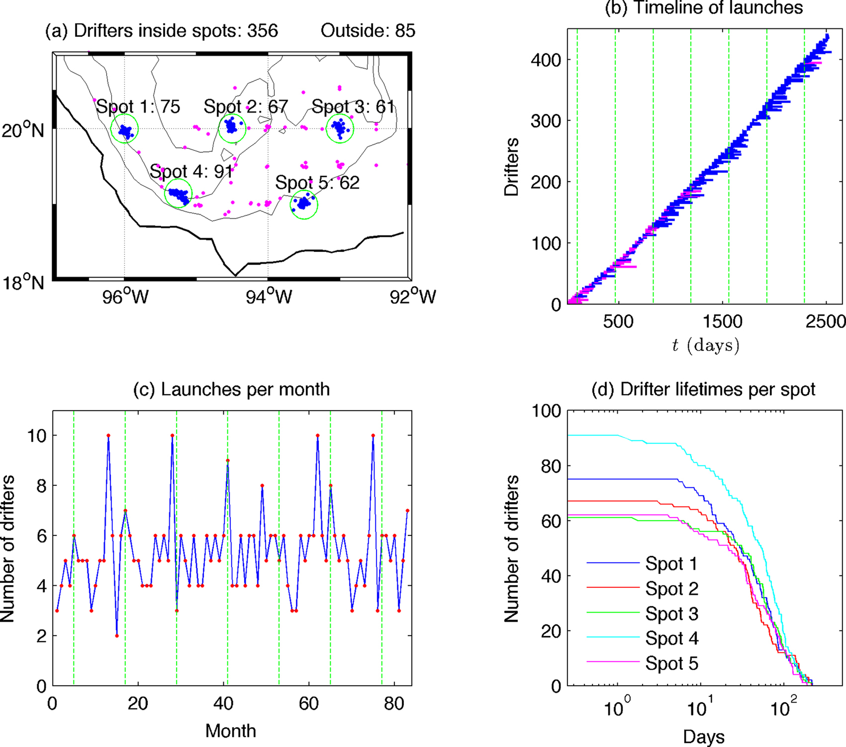
During a 7-year period (starting on September 2007), 441 surface drifters were deployed and tracked in different geographical locations. We mainly focus on 365 drifters launched in five preferential spots, defined by a 20 km radius circle, as shown in figure 1(a). The geographical positions of the spots and the corresponding depth are presented in table 1. In addition, 85 drifters were released in different places over the region, always south of 22°N. The drifters recorded hourly positions, which were interpolated to regular 6 h intervals. The time of release and the lifetimes of each drifter are presented in figure 1(b).
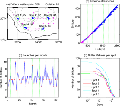
Figure 1 (a) Map of the southern GM showing the five preferential spots where 365 drifters were released (blue dots). The spots are denoted by green circles (20 km radius). Numbers aside the circles indicate the amount of deployments (see also table 1). Magenta dots point out the initial positions of 85 drifters released outside the spots. Topography contours (500, 1500 and 2500 m) are denoted with thin black lines. (b) Time of release of the 441 drifters. Blue and magenta bars correspond with the colored positions in panel (a). Initial time, t = 0 days, is 27 September 2007 and last record is 30 September 2014. Vertical, dashed lines are positioned at January 1st of years 2008 to 2014. (c) Drifter launches per month. Vertical, dashed lines are positioned at January of years 2008 to 2014. (d) Drifter lifetimes. At day zero the number of drifters corresponds to that shown in panel (a).
Download figure:
Standard image High-resolution imageTable 1. Launching spots (see figure 1).
| Spot | Latitude | Longitude | Mean depth (m) | Drifters | Mean lifetime (d) |
|---|---|---|---|---|---|
| 1 | 20°N | 96°W | 1671 | 75 | 60 |
| 2 | 20°N | 94.5°W | 1868 | 67 | 60 |
| 3 | 20°N | 93°W | 1067 | 61 | 71 |
| 4 | 19.15°N | 95.25°W | 1488 | 91 | 64 |
| 5 | 19°N | 93.5°W | 363 | 62 | 62 |
The number of drifters released every month is shown in figure 1(c). In average, there are about 63 launches per year, and between 5 and 6 per month. The lifetimes of the drifters from each spot are shown in figure 1(d). Last value indicates the longest lifetime in each subset. Mean lifetimes are shown in table 1. For the whole data set, including drifters inside and outside spots, the mean lifetime is 62 days with a standard deviation of 47 days. The longest lifetime was 218 days.
2.2. Dispersion ellipses
In order to estimate the dispersion of drifters that start from a common origin we consider dispersion ellipses. The ellipses are calculated with the separations of the particles from the average position or 'center of mass' defined as

where N is the number of particles, is the position in the i-direction of particle k (i = 1, 2 corresponds to zonal and meridional directions, respectively), and t is time. The overbar indicates ensemble average. The dispersion of a cloud of particles with respect to the average position is:

The definition of dispersion (2) is proportional to the average squared separations over all available particle pairs, that is, to relative dispersion (LaCasce 2008).
Dispersion ellipses are equivalent to the so-called variance ellipses, or covariance error ellipses, used in several fields to indicate the dispersion of two sets of data (see e.g. Waterman and Lilly 2015). In our case, the data are the zonal and meridional positions of the drifters, and , at a given time τ. The ellipse is located at the position of the center of mass at that time, and . The semi-axes are proportional to the square root of the relative dispersion components, according to the following expressions:


with c a positive real value that determines the size of the ellipse (we use ). Then this ellipse is rotated an angle θ, with respect to the zonal direction, given by the direction of the eigenvector with the maximum eigenvalue of the positions covariance matrix. Written in terms of a parameter α that runs from 0 to 2π, the ellipse is calculated as:


The time evolution of the dispersion ellipse represents the spread of the particles with respect to the center of mass. Since the drifters were not launched simultaneously, but during a 7-year period, the description is statistical in both space and time.
3. Results
3.1. Circulation features in the southern GM
Here we describe some essential aspects of the mesoscale circulation in the region. Although most of these features have been discussed by several authors, this brief review is necessary because one of the central points in this paper is that the surface dispersion is mainly ruled by different mesoscale processes. Our description here is based on a careful examination of sea surface height maps together with drifter trajectories.
One of the main mesoscale circulations are the anticyclonic Loop Current Eddies (LCEs) arriving from the eastern GM (Vukovich 2007). These structures, with 150 to 300 km in diameter, are shed by the Loop Current and travel westward-southwestward, mainly due to the β-effect (Cushman-Roisin et al 1990). The shedding period of LCEs is very irregular, ranging between 0.5 and 18.5 months (Lugo-Fernández and Leben 2010). The LCEs arrive to the western GM where they interact with other structures and/or collide with the western shelf (Vukovich and Waddell 1991). The collision with the continental topography might lead to several processes, such as the generation of coastal flows, the meridional translation of the eddy, the rebound of the vortex from the western boundary, and the subsequent generation of secondary eddies (Zavala Sansón et al 1998, Zavala Sansón and van Heijst 2000, Sutyrin and Grimshaw 2010).
A second, fundamental structure is the semi-permanent cyclonic gyre at the Bay of Campeche (hereafter referred to as CG), located at the southernmost part of the GM. This feature was reported by various authors (Monreal-Gómez and Salas de León 1997, Vázquez de la Cerda et al 2005), and it was described in more detail by Pérez-Brunius et al (2013).
Figure 2(a) shows an example of a large LCE arriving to the region of study on November 2013, while a CG is well-formed at the south. The CG is centered at about 20°N, 95°W, and it is clearly denoted by drifter trajectories. The LCE moves westward at 24°N approaching the western topography, in such a way that there is almost no interaction with the CG. As a result, most of the drifters in the CG remain trapped in the south.

Figure 2 Drifter trajectories and sea surface height maps showing examples of circulation features in the southern and western GM. The trajectories of a number of drifters correspond to the positions during the month. Black (magenta) dots indicate the beginning (end) of the trajectories. The altimetry surfaces correspond to day 15 in each month. Topography contours (500, 1500, 2500 and 3500 m) are denoted with thin black lines. (a) An anticyclonic Loop Current Eddy (LCE) arrives to the region at a relatively high latitude and barely interacts with the cyclonic gyre (GC) located at the south. (b) A LCE arrives at a lower latitude than in previous case, and strongly interacts with the CG. (c) Example of a narrow, northward flow along the western margin of the GM in the absence of a LCE. (d) Northward advection of drifters due to the presence of secondary cyclones and anticyclones in the western margin of the GM.
Download figure:
Standard image High-resolution imageIn figure 2(b) we present an example in which there is a strong interaction between a LCE and the CG. On January 2012 a LCE arrived to the western side of the GM at a lower latitude than in the previous case, while the CG located at the south is clearly identified by the drifter trajectories. As the LCE approaches the western slope, both structures are strongly deformed. During this interaction, the LCE traps a number of drifters originally located in the CG and pushes them northwards.
Another circulation feature relevant for the surface dispersion is the presence of an intense, along-shore current flowing parallel to the coastline at the western margin of the GM (Zavala-Hidalgo et al 2003, Dubranna et al 2011). This flow is related with the wind stress curl over the northern GM (DiMarco et al 2005). The intensity of the current varies seasonally, being stronger and more frequent during Summer. In figure 2(c) a typical case of this narrow flow is shown during August 2011. Note that this flow might exist regardless of the presence of any LCE or the CG.
There might be more processes in the region playing a role on the export or retention of drifters. Figure 2(d) presents a typical example on July 2013, when the CG is observed with a very circular shape, together with secondary cyclonic and anticyclonic structures at northern latitudes. Some drifters are advected northwards following the circulation of these eddies.
The size of most of the mesoscale features described here (vortices with 100 to 300 km in diameter) is much larger than the size of the spots where the drifters were launched (20 km). Therefore, these locations can be considered as point sources, given that we are focusing on the large-scale spreading of passive tracers released there.
3.2. Trajectories and dispersion ellipses
Now we examine the drifter trajectories from each spot, their average position and the dispersion ellipses at different times. The ellipses show the statistical dispersion from the center of mass at a given time. Recall that the ellipses are centered at the average position of the dispersed drifters, and their orientation indicates the direction of larger dispersion.
Figure 3 presents the results at day 3. At this time we aim at detecting correlated motions near the point sources as the drifters are released (e.g. the presence of a persistent mean flow or the influence of the coastline). Consider first the western spots 1, 2 and 4, which show that the predominant flow is cyclonic. This circulation corresponds to the cyclonic gyre of the Bay of Campeche (CG). In particular, drifters from spot 1 indicate a strong southeastward flow, clearly denoted by the orientation of the dispersion ellipse, followed by zonal dispersion along the coastline from spot 4. The center of mass from the eastern spots 3 and 5 is only slightly directed northwestward, suggesting a weaker influence of the CG.

Figure 3 Drifter trajectories from the spots, trajectories of the center of mass (thick, black lines), and dispersion ellipses (colored on light green) at day 3. The locations of the spots are denoted with a solid, black dot. The drifter trajectories are colored differently for each spot. Red dots indicate the drifter positions at day 3. The position of the center of mass at that day (which defines the center of the ellipses) is represented with an open circle. Topography contours (500, 1500 and 2500 m) are denoted with thin black lines.
Download figure:
Standard image High-resolution imageFigure 4 presents the drifter trajectories and dispersion ellipses at day 30 (panels a to e), a time scale at which the mesoscale features play a fundamental role on the drifter dispersion. The CG is now more clearly depicted by the trajectories starting from the western spots 1, 2 and 4, and it is still visible with trajectories from spot 5 at the east. The drifters from the easternmost spot 3 do not show this behavior, which indicates that the eastern zonal extension of the CG is about 93°W, approximately. In panel (f) the trajectories and the dispersion ellipse of the drifters initially located outside the spots are plotted. The center of mass is initially located at 19.5°N, 94.5°W, approximately, because these drifters were deployed over a wide area in the southern GM (magenta dots in figure 1). The trajectory of the center of mass is directed northwestward, in agreement with the corresponding result from the eastern spots 3 and 5.

Figure 4 Drifter trajectories (blue lines), trajectories of the center of mass (thick, black lines), and dispersion ellipses (colored on light green) at day 30. The locations of the spots are denoted with a solid, plus sign. The drifters released from spots 1 to 5 are shown in panels a to e, respectively. Panel f presents the case of drifters initially launched outside the spots. Red dots indicate the drifter positions at day 30. The position of the center of mass at day 30 is represented with an open circle.
Download figure:
Standard image High-resolution imageThe northwest-southeast orientation of all the ellipses reflects the northward advection of drifters, preferentially along the western side of the GM. A typical situation is that some drifters from all spots are trapped in the CG, and at some point are diverted northward. This happens more frequently with drifters from spot 2, as suggested by the more elongated shape of the dispersion ellipse. Most of such motions are associated with some of the circulation features described in previous section, specially the presence of anticyclonic LCEs arriving from the eastern GM, and wind-driven along-shore flows. The southern CG might be important in this process as well, because the cyclonic circulation accumulates drifters in the south, which are then transported northward during the arrival of a LCE. This description is clear from altimetry images, as shown in figure 2(b).
Another important observation is that the drifters hardly move towards deeper water in the central GM. Furthermore, the drifters practically never penetrate into the Yucatan shelf at the eastern side (Rodríguez Outerelo 2015).
3.3. Dispersion scenarios
We present now the dispersion of drifters from the spots during some particular months that describe two dominant, contrasting scenarios. The main idea is that there are two dispersion patterns that dominate the behavior of surface drifters released in the region: (i) the northward advection of drifters, and (ii) the retention of drifters at the southern GM. These scenarios were distinguished quantitatively by means of two-particle statistics in ZPS16.
The northward advection scenario is identified when 25% of drifters in a given month move beyond 24°N. The blocking scenario is determined when 75% of the drifters remain south from 22°N. Since both cases are essentially different, they can be distinguished by visual inspection of the drifter trajectories during the month. The scenarios are identified during 26 months each, presented in table 2. The selected months might or might not be consecutive through the 84-month period of study. The reason for using some particular months to illustrate the dominant dispersion scenarios, instead of using monthly or seasonal data, is because dispersion is strongly influenced by the already described mesoscale circulation events. This point is further addressed in the Discussion section.
Table 2. Dispersion scenarios.
| Year | Northward advection | Blocking |
|---|---|---|
| 2007 | Dec | Oct |
| 2008 | Feb, Apr, Jun, Nov, Dec | Jul, Aug, Sep, Oct |
| 2009 | Jan, Jun, Jul | Feb, Aug, Oct |
| 2010 | Apr, May, Jun | Feb, Mar, Jul, Aug, Sep |
| 2011 | Apr, Aug | Mar, Jul, Nov |
| 2012 | Jan, May, Jun, Jul, Aug | Mar, Sep |
| 2013 | Feb, May, Jul | Jan, Mar, Sep, Oct, Nov, Dec |
| 2014 | May, Jun, Jul, Aug | Jan, Feb |
In order to show the differences between the two scenarios, figure 5 presents the drifter trajectories in both cases during 30 days, or less for drifters with a shorter lifetime. The first 15-day segments are colored differently than the subsequent section. In the northward advection scenario several drifters move beyond 24°N and even reach the 26°N latitude. As mentioned before, the northward path is mainly along the western margin of the GM. In contrast, for the blocking scenario only a few drifters reach 24°N. Another important difference is the apparent shape and position of the GC: in the northward advection scenario the CG is more compact and located more to the west, while in the blocking case the CG is wider and centered more to the east.
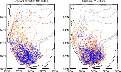
Figure 5 Drifter trajectories showing the dominant dispersion scenarios: (a) Northward advection. (b) Blocking. The drifter trajectories start in one of the months that define the dispersion scenarios in table 2. The maximum duration of the trajectories is 30 days. The first 15 days are colored in blue; subsequent days are colored in orange. Small, black (red) dots indicate the initial (final) position of drifters. Topography contours (500, 1500, 2500 and 3500 m) are denoted with thin black lines.
Download figure:
Standard image High-resolution imageFigures 6 and 7 show the drifter trajectories and dispersion ellipses for the northward advection and blocking scenarios, respectively. The first feature to notice is that the dispersion ellipses in the northward advection scenario are indeed much more elongated in the meridional direction than those in the blocking scenario. The ellipses in the latter case are almost circular, except in spot 1. The shape of the ellipses can be interpreted as a graphical representation of the anisotropy of relative dispersion during the northward advection scenario, contrasting with the isotropy observed during the blocking scenario.

Figure 6 Same as in figure 4 but now for drifters released during the northward advection scenario (26 months, see table 2).
Download figure:
Standard image High-resolution image
Figure 7 Same as in Figure 4 but now for drifters released during the blocking scenario (26 months, see table 2).
Download figure:
Standard image High-resolution imageA second observation is that the north-south elongation of the ellipses in the northward advection scenario is more pronounced for drifters starting from spot 2, in the central region. This is interpreted in terms of the presence of LCEs in the southern GM. Drifters released from this spot might be trapped during the arrival of a LCE and then strongly advected northwards by the western flank of the vortex.
Another important point is that drifters from the eastern spot 3 are dispersed northwestward on average, regardless of the dispersion scenario (the dispersion ellipses in figures 6(c) and 7(c) are very similar). This is an indication that dispersion from the eastern part of the region tends to be northwestward in general, as observed with the full set of drifters in figure 4.
4. Discussion and Conclusions
The drifter trajectories and dispersion ellipses provide a statistical overview of the possible paths and areas covered by the drifters. We discuss these results from three points of view related with (i) the methodology to represent the drifter dispersion from a point source, (ii) the environmental perspective, and (iii) the dispersion scenarios. Possible readers of this paper, with different expertise and interests, might focus on one of these approaches.
- (i)Dispersion ellipses are a simple statistical tool that reflect the spread of drifters from a point source. The construction is based on the same principles to calculate ellipses of variability, commonly used to represent the statistical dispersion of observed data. In oceanographical applications, variance ellipses are often used to describe the variability of ocean data at a fixed point, such as the horizontal velocities measured in moorings (e.g. Sheinbaum et al 2010). Another important application is to describe the eddy vorticity flux divergence by means of the horizontal velocity covariance matrix (Waterman and Lilly 2015). Recently, Rypina et al (2012) reported the so-called 'spreading ellipses', which are essentially equivalent to the dispersion ellipses used here. An important difference is that the spreading ellipses are referred to geographical bins in a regular grid, in order to represent the direction of maximum spreading at fixed points. Here, in contrast, the dispersion ellipse is located at the moving center of mass of the drifters, and its size grows as the drifters are dispersed. Thus, the dispersion ellipse effectively tracks the evolution of a two-dimensional patch of a tracer released from a specific location.It must be recalled that the drifters considered here are not released simultaneously. Therefore, the simple shape of the ellipse reflects their statistical dispersion. The eccentricity of the dispersion ellipse represents the relative importance of the dispersion components, and its orientation indicates the direction of maximum dispersion. The size of the dispersion ellipse is arbitrary, because it represents a confidence area within which a chosen percentage of the data is contained. For instance, if the drifter displacements with respect to the center of mass have a nearly normal distribution, then a constant in the definition of the semi-axes (3) and (4) implies that 95% of the final positions are within the ellipse, approximately.
- (ii)The results are oriented to give useful information from an environmental point of view. Such a perspective is based on the deployment of several drifters from the preferential spots, so their dispersion represent the area where a passive tracer is most likely to be found a given time after it has been released from the point source. Since there are no chemical or biological degradation processes affecting the drifter distributions, their dispersion can be considered as the maximum spread of the passive contaminant. This is the basic rationale in contingency plans in general, and in particular for large oil spills (Boufadel and Geng 2014). Thus, the results can be interpreted as part of the risk assessment typically considered in early stages of contingency plans for marine oil spills (ITOPF 2016).When discussing the evaluation of the transport and fate of oil, Boufadel and Xeng (2014) made an important remark in their short note, namely, that 'seasonal averages should be discouraged unless proven otherwise'. We agree with this statement when considering dispersion in the southern GM, because seasonal averages might obscure the behavior of a set of tracers released from a point source. The reason is that the dispersion mechanisms are closely related with mesoscale circulation features, which might be present during any time of the year, and last from some weeks to a few months. The complexity of the turbulent dispersion problem stems from the fact that different circulation processes might occur simultaneously and interact with each other. In some cases they might reinforce or inhibit the dispersion of drifters. Therefore, when using seasonal averages the dispersive effects associated to these circulation events might be blurred.
- (iii)During the northward advection scenario, the dispersion ellipses are clearly more elongated than in the blocking scenario. The identification of these two contrasting cases seems adequate for the GM, but it cannot be a general rule. In other locations it might be more appropriate to analyze seasonal data or some other period to describe characteristic patterns of dispersion. A seasonal component is not discarded here either, because we have only analyzed an 84-month database of drifter trajectories. Another relevant point is that there might be more dispersion scenarios or variations of those presented here. Therefore, the present description might serve as a starting point to explore more dispersion scenarios.

The results may also be used to make preliminary estimations in dispersion problems. Suppose that a certain contaminant is continuously released somewhere in the region. Then it might be relevant to estimate the occurrence of one of the contrasting scenarios described here. The presence of LCEs and the development of the CG could be determined by examining altimetry maps or with the help of operational numerical simulations. Thus, depending on the position, size and strength of these structures, it might be possible to infer the occurrence of one of the dispersion scenarios: the northward advection of a large number of tracers or their retention at the south. Certainly, the prediction might fail when the LCEs or the CG are not present or when there are additional structures or complicated patterns not considered here. Despite this, we consider that the information described in this study provides useful tools for both diagnostics and prognostics of the spread of passive tracers near the surface of the GM.
Acknowledgments
Surface drifter data were obtained from a project funded by PEMEX Exploración y Producción under contracts SAP nos. 428217896, 428218855, and 428229851, with support of the Eddy Watch group from Horizon Marine Inc. We thank Paula García and Argelia Ronquillo for quality control and post-processing of the drifter data. This research is a contribution of the Gulf of Mexico Research Consortium (CIGoM), funded by the National Council of Science and Technology of Mexico—Secretariat of Energy -Hidrocarbons Trust, project 201441.