Non-closure of the surface energy balance explained by phase difference between vertical velocity and scalars of large atmospheric eddies

The post-field data processing procedures are documented elsewhere (Zhang et al 2010, Zhang and Liu 2014, Gao et al 2016). Briefly, these procedures include: 1) removing physically impossible values and spikes from the time series; 2) double rotation for the sonic anemometer measured w (Kaimal and Finnigan 1994); 3) calculation of averages, variances and covariances using a 30 min block average; 4) sonic temperature correction (Schotanus et al 1983, Liu et al 2001), oxygen cross sensitivity correction for KH20 (Tanner et al 1993), density correction applied to LE (Webb et al 1980), and correction for flux attenuation due to spatial separation of CSAT3 and KH20 (Oncley et al 2007); and 5) quality check for stationary and developed turbulent conditions (Foken et al 2004).

Using the method in Liebethal et al (2005) and Oncley et al (2007), G₀ was determined from measurements by heat flux plates at a depth z_p and the heat stored in the soil layer between the surface and z_p,

$$\begin{equation} G_0 = c_{\text{soil}} z_\text{p} \frac{{\text{d}T_{\text{soil}} }}{{\text{d}t}} + G(z_\text{p} ), \end{equation} \tag{ 1 }$$

where T_soil is the mean soil temperature between the surface and z_p, and c_soil is the volumetric heat capacity of moist soil calculated by:

$$\begin{equation} c_{\text{soil}} = Q_{\text{soil}} (\rho c)_{\text{water}} + (\rho c)_{\text{soil,dry}} , \end{equation} \tag{ 2 }$$

where (ρc)_water and (ρc)_soil,dry are the volumetric heat capacities of water (4.2 × 10⁶ J m⁻³ K⁻¹) and soil minerals (2.5 × 10⁶ J m⁻³ K⁻¹), respectively, and Q_soil is the layer-averaged volumetric water content. Unlike soil heat conductivity that can vary with the particular configuration of soil pore structure, soil particle contact areas and water bridge configurations between them, specific heat capacities vary linearly in proportion to the constituent material. Previous studies suggested that the method described above is one of the highly recommended methods depending on data availability (Liebethal et al 2005, Russell et al 2015).

To quantify the phase difference between low-frequency series of w, q, and T caused by large eddies, we first detected and extracted large eddies (i.e. low-frequency structures) from the 10 Hz time series data. Traditionally, Fourier-based filters and wavelet decompositions were deployed to separate large eddies from an oscillatory signal using pre-determined basis functions. Non-linear and non-stationary nature of turbulence could prevent successful implementation of the traditional methods on turbulence decomposition because both Fourier and wavelet transforms cannot readily accommodate non-linear and non-stationary series without 'extra' ad-hoc post-processing (Huang et al 1998, Huang and Wu 2008). Compared to Fourier-based filters and wavelet decompositions, the empirical mode decomposition (EMD) is adaptive and has high locality, and therefore capable of handling some of the non-linear and non-stationary occurrences that are ubiquitous in turbulence data (Huang et al 1998, Huang and Wu 2008). EMD has been favored in several atmospheric boundary layer (ABL) studies (Hong et al 2010, Barnhart et al 2012, Wang et al 2013, Gao et al 2016). The ensemble empirical mode decomposition (EEMD) (Wu and Huang 2009), a method based on EMD (Huang et al 1998, Huang and Wu 2008) for time series analysis, was adopted here. Using a sifting process, EEMD decomposes a time series x(t) into a finite set of amplitude-frequency modulated oscillatory components C_j,x (j = 1, 2, ..., n) and a residual r_n(t). This residual is a time series that is either monotonic or containing only one extremum from which no more oscillatory components can be further extracted. Hence,

$$\begin{equation} x(t) = r_n (t) + \sum\nolimits_{j = 1}^n {C_{j,x} (t).} \end{equation} \tag{ 3 }$$

To ensure the equivalence of variances and covariances calculated from all extracted components (i.e. C_j,x and r_n) and the post-field data processing, the EEMD was applied to each 30 min time series data of w', q' and T'. The prime denotes the turbulent fluctuations relative to the 30 min block average after despiking and double rotation (i.e. steps 1 and 2 in section 3.1). EEMD can only sift out oscillatory components that differ in period by more than a factor of two (Huang et al 1998, Huang and Wu 2008, Barnhart et al 2012). For each 30 min time series run, thirteen oscillatory components (i.e. n = 13) were extracted with one overall residual r₁₃, marked as the fourteenth component (C_14,x). The residual was included because it still contributes to the total variance and possibly covariance as compared to the traditional post-field data processing (Barnhart et al 2012). Each oscillatory component has its own characteristic frequency (Wang et al 2013). Since all time-domain components are additive, the sum of certain oscillatory components can be interpreted as large eddies if a critical frequency is identified and assigned as a delineator of large scales (Wang et al 2013).

Several methods for identifying a critical frequency have been proposed to separate large eddies from small eddies, including a spectral gap in the v spectra (Cava and Katul 2008), a copsectral gap in uw and wT cospectra (Vickers and Mahrt 2003), and the first clearly identified maximum in wavelet variance spectrum (Thomas and Foken 2005, Barthlott et al 2007, Zhang et al 2011). In the EBEX-2000 dataset, a spectral gap at about 0.02 Hz did exist for some cases in their v spectra (Zhang et al 2010, Gao et al 2016). Zhang et al (2011) calculated the characteristic scales of coherent structures (i.e. large eddies) under different atmospheric stability conditions using the same dataset, and found that the averaged frequency for dominant large eddies was also about 0.02 Hz during the daytime for this site. Based on these previous studies, oscillatory components with the mean frequencies smaller than 0.02 Hz are labeled as large eddies (i.e. $x^\prime_l = \sum\nolimits_{j = 19}^{14} {Cj,x} ,$, where x = w, q, and t, and l refers to large eddies for x), and larger than 0.02 Hz as small eddies (i.e. $x^\prime_s = \sum\nolimits_{j = 1}^8 {Cj,x} ,$, where s refers to small eddies for x). Different tests indicated that the selection of the critical frequency only has minor effects on quantifying phase difference and flux contribution. Turbulent fluxes of large and small eddies were corrected following step 4 in the post-field data processing (section 3.1).

There are three methods for estimating phase difference between different quantities: Fourier transform, wavelet transform, and Hilbert transform (Stull 1988, Quiroga et al 2002, Grinsted et al 2004). Separate tests (not shown here) indicated that these three methods resulted in similar phase difference when sinusoidal signals with known phase difference were processed. Nevertheless, taking into account the concerns in previous studies that both Fourier and wavelet transforms may induce uncertainty when non-linear and non-stationary data are processed, the Hilbert transform was deemed better suited for this purpose (Huang et al 1998, Quiroga et al 2002).

For a signal x(t), its Hilbert transform, $\hat x\left( t \right)$, is given as,

$$\begin{equation} \hat x(t) = \frac{1}{\pi }PV\int_{ - \infty }^\infty {\frac{{x(\tau )}}{{t - \tau }}\text{d}\tau ,} \end{equation} \tag{ 4 }$$

where PV denotes a Cauchy principle value integral. Mathematically, the HT is a phase shift of the original signal by −90°. Thus, an analytic signal can be constructed from the signal and its Hilbert transform as

$$\begin{equation} z^x (t) = x(t) + i\hat x(t) = A(t)\text{e}^{\text{i}\Phi (t)} , \end{equation} \tag{ 5 }$$

$$\begin{equation} A(t) = (x^2 + \hat x^2 )^{\tfrac{1}{2}}, \end{equation} \tag{ 6 }$$

$$\begin{equation} \Phi (t) = \tan ^{ - 1} \left( {\frac{{\hat x}}{x}} \right), \end{equation} \tag{ 7 }$$

where $i = \sqrt { - 1}$, A is the instantaneous amplitude, and Φ is the instantaneous phase function. Because the Hilbert transform is by construct sensitive to instantaneous phase shifts encoded as t − τ in equation (4), it offers advantages over wavelet or Fourier methods.

Similar to Fourier and wavelet cross spectrum, the Hilbert cross spectrum of two signals x(t) and y(t) is defined as

$$\begin{equation} HCS^{xy} (t) = z^{x*} (t)\cdot z^y (t), \end{equation} \tag{ 8 }$$

where ⁎ denotes complex conjugation. The instantaneous Hilbert phase difference between two signals is obtained as

$$\begin{equation} \Phi _{\text{diff}} (t) = \tan ^{ - 1} \left( {\frac{{\text{Im}\;\text{[}HCS^{xy} \text{(}t\text{)]}}}{{\text{Re[}HCS^{xy} \text{(}t\text{)]}}}} \right), \end{equation} \tag{ 9 }$$

where Im and Re denote the imaginary and real parts of the Hilbert cross spectrum, respectively. Here, the time-averaged $\Phi _{\text{diff}} \left( t \right)$ associated with large eddies is used to represent the phase difference between $w_l^\prime$ and $q_l^\prime$ for each run.

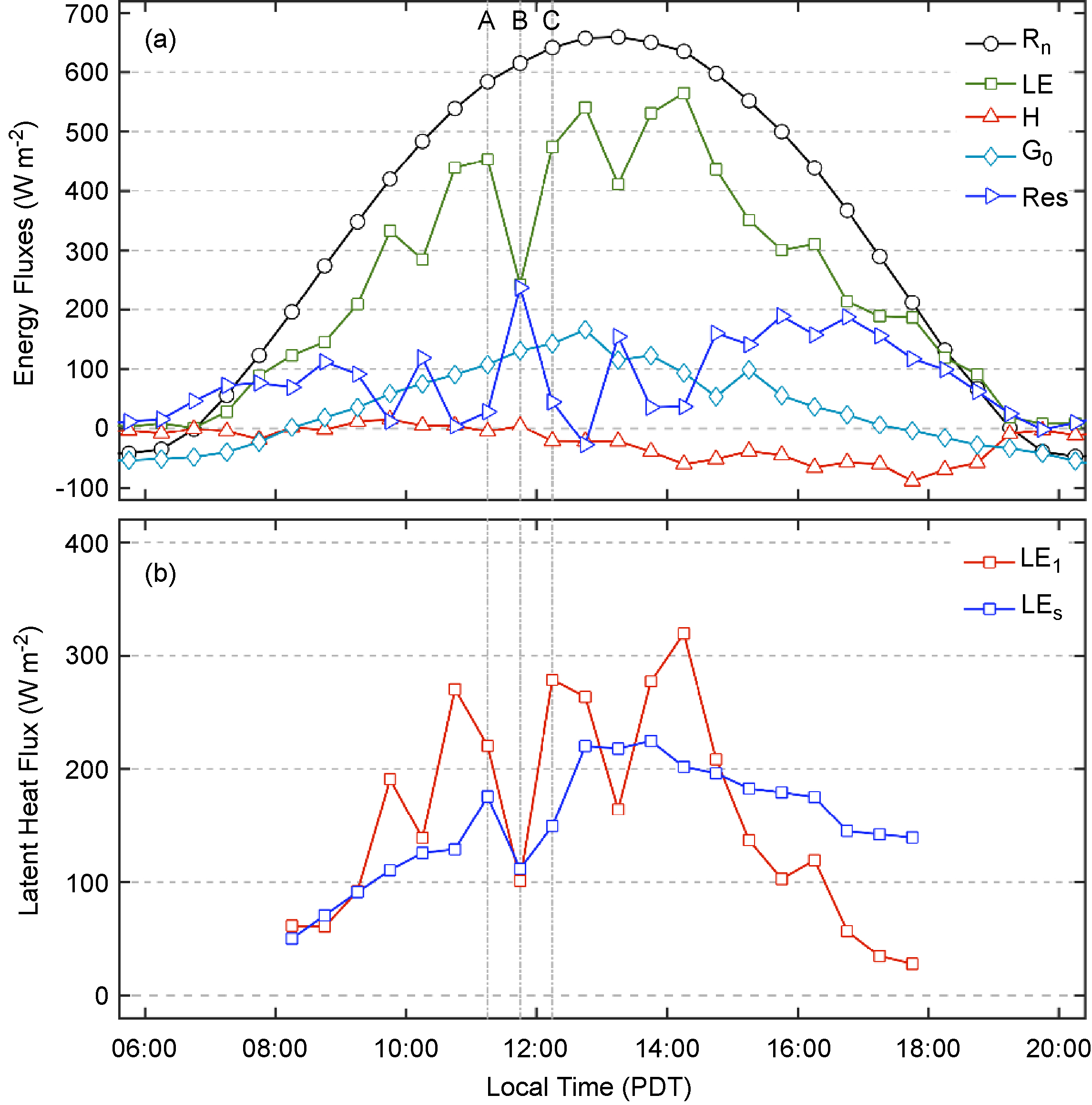
Typical daytime 30 min mean LE in EBEX showed large point-to-point variations with the varying magnitudes of over 200 W m⁻², especially during the late morning to early afternoon (figure 1(a)). The variations suggested that other external forcing beyond R_n affected the evapotranspiration, because R_n followed a nearly ideal sine shape, with a maximum value of about 700 W m⁻² at 13:00 PDT (local noon; figure 1(a)). When partitioning LE into flux contributions by large eddies (i.e. LE_l caused by $w_l^\prime$ and $q_l^\prime$) and small eddies (i.e. LE_s caused by $w_s^\prime$ and $q_s^\prime$), more pronounced point-to-point variations in LE_l was noted compared to LE_s during the late morning to early afternoon. In the late afternoon after 14:00 PDT, LE_l showed a large decreasing trend and approached zero by about 18:00 PDT, whereas LE_s exhibited a small decreasing trend during the entire afternoon (figure 1(b)). The decreased LE_l was largely attributed to horizontal advection under warm (dry)-to-cool (wet) transition from the upstream drier patches to the wet cotton field (Oncley et al 2007, Zhang et al 2010), leading to a reduced surface energy balance closure in the afternoon than in the morning at the study site.

Zoom In Zoom Out Reset image size

As shown in table 1, a case study is featured illustrating that despite the comparable magnitudes between low-frequency signals of w and those of q caused by large eddies (i.e. $w_l^\prime$ and $q_l^\prime$), the phase difference between them led to large reduction in the contribution of large eddies to LE. Would this conclusion be generally applicable to explain the influence of large eddies on ASL turbulence and energy balance non-closure? How do simultaneous changes in both magnitudes and phase difference between two quantities (i.e. $w_l^\prime$ and $q_l^\prime$) modulate the influence of large eddies on turbulent fluxes? To make our calculation manageable, the daytime data in EBEX were divided into five groups according to the ranges of the magnitudes of $w_l^\prime$ ($\left( {A_l^w } \right)$) and $q_l^\prime$ ($\left( {A_q^l } \right)$). Each group consists of 30 min data points with $A_l^w A_l^q$ being located within a magnitude range of 0–0.1, 0.1–0.15, 0.15–0.2, 0.2–0.25, and > 0.25 g m⁻² s⁻¹ (= m s⁻¹ g m⁻³). Figure 2(a) shows that for all five groups, LE_l generally decreased with the increased phase difference between $w_l^\prime$ and $q_l^\prime$, though the decrease trends of LE_l with the increasing phase difference were different for the groups. The larger the magnitude ranges, the greater the slopes, suggesting that the flux contribution from more energetic large eddies was more sensitive to changes in phase shifts. Given the same phase difference, LE_l was greater for the larger magnitude ranges, reflecting that the $w_l^\prime$ and $q_l^\prime$ magnitude affected flux contributions of large eddies. Figure 2(a) also indicates that LE_l varied across larger ranges under smaller phase difference (e.g. $\left| {\Phi _{\text{diff}} } \right| = 40^\circ$) than larger phase difference (e.g. $\left| {\Phi _{\text{diff}} } \right| = 80^\circ$). LE_l from all groups converged to smaller values when phase differences became larger, and all groups approached zero when $\left| {\Phi _{\text{diff}} } \right|$ became 90°. When $w_l^\prime$ and $q_l^\prime$ became out of phase, the large eddies contributed little to LE no matter how energetic large eddies are (as quantified by their $w_l^\prime$ and $q_l^\prime$ magnitudes). For the study site, H was relatively small and even negative during the daytime, while it is still true that H contributed by large eddies (i.e. $w_l^\prime$ and $T_l^\prime$) decreased with the increasing phase difference given the comparable magnitudes of $A_l^w A_l^T$ (figure S1 available at stacks.iop.org/ERL/12/034025/mmedia). We also computed the flux contribution and phase difference between small eddies of w and q (i.e. $w_s^\prime$ and $q_s^\prime$). The mean absolute phase difference between $w_s^\prime$ and $q_s^\prime$ only varied within a small range of 60°−78° because small eddies are becoming locally isotropic and de-correlated because of the action of pressure-velocity and pressure-scalar interactions (Li and Bou-Zeid 2011). As a result, the decrease in LE_s with the increase in phase difference between $w_s^\prime$ and $q_s^\prime$ was not as obvious as that for the large eddies (figure S2).

Table 1. Characteristics of large eddies for the three cases A (11:00–11:30 PDT), B (11:30−12:00 PDT), and C (12:00–12:30 PDT), respectively. LE_l is the latent heat flux contributed by large eddies. $A_l^\w$ ± SD and $A_l^\q$ ± SD are mean and standard deviation of the instantaneous amplitudes for $w_l^\prime$ and $q_l^\prime$, respectively. $\left| {\Phi _{\text{diff}} } \right|$ ± SD is mean and standard deviation of the absolute instantaneous phase difference between $w_l^\prime$ and $q_l^\prime$ in units of degree. ΔLE_l is the increase of the latent heat flux contributed by large eddies by artificially modifying the phase difference between $w_l^\prime$ and $q_l^\prime$ with their amplitudes intact by using Fourier transform and its inverse transform.

Cases	Rn − G0 (W m−2)	LE (W m−2)	H (W m−2)	LEl (W m−2)	$A_w^q$ ± SD (m s−1)	$A_l^q$ ± SD (g m−3)	$\left| {\Phi _{\text{diff}} } \right|$ ± SD (deg)	ΔLEl (W m−2)
A	476.8	453.3	−5.1	220.3	0.16 ± 0.09	1.31 ± 0.69	49.6 ± 47.9	49.5
B	484.5	242.7	4.4	101.2	0.19 ± 0.12	1.40 ± 0.69	74.1 ± 49.7	180.9
C	498.2	474.8	−21.5	278.5	0.17 ± 0.09	1.51 ± 0.73	43.6 ± 40.5	78.5

Zoom In Zoom Out Reset image size

Since enlarged phase difference between $w_l^\prime$ and $q_l^\prime$ led to the reduction in LE_l, it is expected that the surface energy balance closure was degraded with enlarged phase difference. This statement is confirmed by figure 2(b) in which the ratio of the sum of the turbulent fluxes to the available energy (i.e. (H + LE)/(R_n− G₀)) decreased with the increase in phase difference between $w_s^\prime$ and $q_s^\prime$. As stated above, LE_l increased with $A_l^w A_l^q$ at fixed $\left| {\Phi _{\text{diff}} } \right|$. Therefore, (H + LE)/(R_n− G₀) also increased with $A_l^w A_l^q$ given the same phase difference (figure 2(c)). To demonstrate whether the reduced phase difference alone is able to improve the closure for the dataset in EBEX-2000 presented in figure 2(d), we artificially modified the phase difference between $w_l^\prime$ and $q_l^\prime$ ($T_l^\prime$) with their amplitudes intact by using Fourier transform, as the inverse Fourier transform of a signal equals to the original signal. For instance, the phase of $q_l^\prime$ was artificially set to the phase of $w_l^\prime$ but amplitudes were not altered. This artificial adjustment would cause an increase of about 27% in LE (figure S3, table S1). For $w_l^\prime$ and $T_l^\prime$, under unstable conditions, the phase of $T_l^\prime$ was artificially set to the phase of $w_l^\prime$ but, under stable conditions, the phase of $T_l^\prime$ was artificially set to be out of phase with $w_l^\prime$ so that $w_l^\prime$ and $T_l^\prime$ would have a negative flux contribution. The linear regression between the original H and the modified H has a slope of 1.25 ± 0.02 and an intercept of (2.02 ± 0.71) W m⁻² with an absolute value for R² of 0.94 (figure S3, table S1). After the modification of phase difference for all data points, the surface energy balance closure improved significantly (P < 0.001) from 0.77 ± 0.18 to 0.97 ± 0.20 with similar values of R² as shown in table 2. The above tests suggest that phase differences between $w_l^\prime$ and $q_l^\prime$ were responsible for a significant portion of the energy balance non-closure.

What causes these phase differences in large eddies is difficult to discern from single-point time series analysis. However, a number of conjectures may be offered. The daytime unstable ASL over moist landscapes is statistically predominated by upward warm/moist (e.g. $w_s^\prime > 0$ and $q_s^\prime > 0$) and downward cool/dry (e.g. $w_s^\prime < 0$ and $q_s^\prime < 0$) turbulent eddies when their size is commensurate with the measurement height z_m, leading to positive H and LE (e.g. $\overline {\left( { + w_s^\prime } \right)\left( { + q_s^\prime } \right)} > 0$ and $\overline {\left( { - w_s^\prime } \right)\left( { - q_s^\prime } \right)} > 0$) in the absence of advection. If large eddies (i.e. those much larger than z_m) have the same attributes as the small-scale turbulence and disturbed the ASL, these upward warm/moist (e.g. $w_l^\prime > 0$ and $q_l^\prime > 0$) and downward cool/dry (e.g. $w_l^\prime < 0$ and $q_l^\prime < 0$) large eddies would contribute positively to sensible and latent heat fluxes (e.g. $\overline {\left( { + w_l^\prime } \right)\left( { + q_l^\prime } \right)} > 0$ and $\overline {\left( { - w_l^\prime } \right)\left( { - q_l^\prime } \right)} > 0$). Under this circumstance, large-scale changes in time-series of vertical wind velocity and scalars (e.g. water vapor density) are considered to be in phase (i.e. phase difference $\left| {\Phi _{\text{diff}} } \right| = 0^\circ$). If downward moving large eddies carry warm/moist air masses (e.g. $w_l^\prime < 0$ and $q_l^\prime > 0$), these large eddies would contribute negatively to sensible and latent heat fluxes (e.g. $\overline {\left( { - w_l^\prime } \right)\left( { + q_l^\prime } \right)} > 0$). In this case, large-scale changes in the time-series of vertical wind velocity and scalars (e.g. water vapor density) for large eddies are considered to be perfectly out-of-phase (i.e. $\left| {\Phi \text{diff}} \right| = 180^\circ$). In reality, large-scale phase between vertical wind velocity and scalars varies from 0° to 180°. Hence, in the absence of advection and for the case of entrainment and storage (leading to a time lag) within the much studied convective ABL, it follows that $\left| {\Phi \text{diff}} \right|$ will be finite.

The problem of horizontal advection of dry air onto a wet surface is of particular interest here because its qualitative effects on the energy balance non-closure is predictable and serves as another test case for understanding the genesis of $\left| {\Phi \text{diff}} \right|$. In the presence of advection, the mean continuity equation for water vapor density at z_m above a canopy of height h reduces to

$$\begin{equation} U\frac{{\partial \overline q }}{{\partial x}} \approx - \frac{{\partial \overline {w^\prime q^\prime} }}{{\partial z}}, \end{equation} \tag{ 10 }$$

where U is the mean longitudinal wind speed and x and y are the longitudinal and vertical directions, respectively. The overbar denotes the 30 min average. Because advection of dry air onto a wet surface generates a positive $\partial \overline q /\partial x$, the $U\left( {\partial \overline q /\partial x} \right)$ is always positive (as is the case here) and $\overline {w^\prime q^\prime } \left( {z_m } \right) = \overline {w^\prime q^\prime } \left( h \right) - \int_h^{z_m } {U\left( {\frac{{\partial \overline q }}{{\partial x}}} \right)\text{d}z.}$ Because $\overline {w^\prime q^\prime } \left( {z_m } \right)\left| { < \overline {w^\prime q^\prime } \left( h \right)} \right|$, the proper energy balance residual $= R_n - G_0 - L_v \overline {w^\prime q^\prime } (h)$is expected to be smaller than the measured $= R_n - G_0 - L_v \overline {w^\prime q^\prime } (z_m )$, where L_v is the latent heat of vaporization of water. The $\left| {\Phi \text{diff}} \right|$ for these advective conditions is shown in figure 3. The stability parameter ζ is calculated using ζ =(z_m − d)/L, where d is the zero-plane displacement and L is the Obukhov length. The analysis in figure 3 demonstrates that advective conditions did result in negative sensible heat flux (i.e. ζ > 0 for daytime values), increased energy balance residual, and a correlation coefficient between air temperature and water vapor density that is sufficiently negative consistent with expectations of dry and warm air parcels advecting onto the sensor. In these cases, the measured $\overline {q\prime^2 }$ appears larger than that predicted from surface fluxes represented by $q_* = - \overline {w^{\prime}q^{\prime}} \left( {z_m } \right)/u_*$, where $q_*$ and $u_*$ are the scale for water vapor density and the friction velocity, respectively, and those large excursions are associated with increases in $\left| {\Phi _{\text{diff}} } \right|$. Hence, it can be surmised that advection increases the phase between $w_l^\prime$ and $q_l^\prime$ presumably due to finite travel time of dry and warm air parcels to the sensor location. Both entrainment/storage or advective travel time lead to increases in $\left| {\Phi _{\text{diff}} } \right|$ with afternoon advection having a more pronounced impact on the energy balance non-closure (i.e. larger $\left| {\Phi _{\text{diff}} } \right|$).

Zoom In Zoom Out Reset image size