

Abstract
The land-use regression (LUR) approach to estimate the levels of ambient air pollutants is becoming popular due to its high validity in predicting small-area variations. However, only a few studies have been conducted in Asian countries, and much less research has been conducted on comparing the performances and applied estimates of different exposure assessments including LUR. The main objectives of the current study were to conduct nitrogen dioxide (NO2) exposure assessment with four methods including LUR in the Republic of Korea, to compare the model performances, and to estimate the empirical NO2 exposures of a cohort.
The study population was defined as the year 2010 participants of a government-supported cohort established for bio-monitoring in Ulsan, Republic of Korea. The annual ambient NO2 exposures of the 969 study participants were estimated with LUR, nearest station, inverse distance weighting, and ordinary kriging. Modeling was based on the annual NO2 average, traffic-related data, land-use data, and altitude of the 13 regularly monitored stations.
The final LUR model indicated that area of transportation, distance to residential area, and area of wetland were important predictors of NO2. The LUR model explained 85.8% of the variation observed in the 13 monitoring stations of the year 2009. The LUR model outperformed the others based on leave-one out cross-validation comparing the correlations and root-mean square error. All NO2 estimates ranged from 11.3–18.0 ppb, with that of LUR having the widest range. The NO2 exposure levels of the residents differed by demographics. However, the average was below the national annual guidelines of the Republic of Korea (30 ppb).
The LUR models showed high performances in an industrial city in the Republic of Korea, despite the small sample size and limited data. Our findings suggest that the LUR method may be useful in similar settings in Asian countries where the target region is small and availability of data is low.
Export citation and abstract BibTeX RIS

Original content from this work may be used under the terms of the Creative Commons Attribution 3.0 licence.
Any further distribution of this work must maintain attribution to the author(s) and the title of the work, journal citation and DOI.
1. Introduction
A valid exposure assessment is important in epidemiological studies to analyze the effects of environmental exposure on adverse health outcomes (Rothman et al 2008). Invalid exposure assessment could lead to biased estimates. The most accurate measures can be achieved by directly performing personal monitoring or methods such as biomarkers. However, measuring personal exposure or biomarkers is sometimes infeasible due to the substantial time, physical, and financial efforts needed for such measurement. As a consequence, the spatiotemporal characteristics of exposure and health data do not align in many epidemiological studies, which introduce the potential for measurement errors (Gryparis et al 2009).
Regarding the difficulties in implementing individual monitoring, alternative methods of exposure estimation with surrogate measures and spatial modeling are becoming more popular in examining the relationship between air pollution and adverse health outcomes (Son et al 2010). Common methods for estimating the air pollution exposure levels of an individual are the use of: the concentration of a monitoring station closest to the residential address of an individual; the averaged concentration of monitoring stations within a geographic boundary; surrogate measures of air pollution such as distance to nearest roads or length of roads within a specified boundary; and estimates produced by models such as kriging or inverse distance weighting (IDW).
Among these methods, exposure assessments on a spatially aggregated level fail to take spatial heterogeneity into account (Son et al 2010). To overcome such challenges, methods of spatial interpolation, dispersion models, integrated meteorological-emission models, and land-use regression (LUR) have been introduced. Spatial interpolation methods (e.g. kriging and IDW) take into account spatial heterogeneity by assuming that the concentration level of an unknown spot is similar to the concentrations of nearby known values. However, such approaches do not consider that air pollution concentrations are highly dependent on stationary and mobile sources, which may act as a source of measurement error. Both dispersion and integrated meteorological-emission models are generally considered to be more reliable and transferable, but are costly and difficult to implement due to the vast amount of input data and complicated procedures (Jerrett et al 2005, Peng and Bell 2010).
In line with such issues, LUR has been suggested as an alternative methodology to enhance exposure assessment in terms of spatiotemporal heterogeneity. This method estimates pollution concentration at a given location by generating a regression model utilizing data of surrounding land use, traffic characteristics, and meteorology (Briggs et al 1997). The LUR method is known to have high validity, useful in detecting small-area variations, and is comparatively easy to implement relative to some other approaches (Ryan and LeMasters 2007). The annual concentrations of ambient air nitrogen dioxide (NO2) and nitrogen oxides (NOx) are frequently the subject of prediction with LUR (Beelen et al 2013), because they originate from transportation. Transportation is a known risk factor for many adverse health outcomes (e.g. respiratory symptoms/diseases, otitis media, hospital admissions, and mortality) (D'Amato, 2002, Latza et al 2009, Lee et al 2013, Nitschke 1999). Improved exposure assessment of NO2 may enable us to generate more valid risk estimates, and therefore improve understanding of the health effects of NO2.
Despite the benefits of LUR modeling in NO2 estimation, most study areas of previous literature are limited to western countries (Beelen et al 2013, Hoek et al 2008), with limited study in Asian countries. Most of the previous studies in Asia had been conducted in China (Chen et al 2010, Chen et al 2012, Li et al 2015, Liu et al 2015), with a few in Japan (Kashima et al 2009), the Republic of Korea (Lee et al 2012, Kim and Guldmann 2015), and Taiwan (Lee et al 2014). Also, only a few studies have been conducted on comparing the exposure estimates of LUR modeling with that of the conventionally used exposure assessment methods.
In the current study, our major aims were to compare multiple exposure assessment methods that are widely in use and to apply the best performing model to estimate the annual NO2 exposure levels of a cohort in an industrial city in the Republic of Korea. For this purpose, three conventionally used exposure assessment methods (i.e. IDW, kriging, and nearest monitoring station) and one advancing exposure assessment method (i.e. LUR) were used to build NO2 prediction models in Ulsan, an industrial city in the Republic of Korea. The validity of each model was compared, and the best performing model was used to empirically estimate the NO2 exposure of the subjects in a cohort in Ulsan.
2. Materials and methods
2.1. Study population and air pollution data
The study participants were restricted to the participants of the Ulsan cohort in the year 2010, whose exact residential address was known. Ulsan is a highly industrialized city located in the southeastern part of the Korean Peninsula. Ulsan is considered a symbol of economic development in the Republic of Korea, with two large industrial complexes (the Ulsan petro-chemical complex and the Ulsan Mipo industrial complex) within the borders of the city. The Ulsan cohort is a government-supported study established in 2003 to monitor exposure levels and biomarkers of environmental pollutants in the residents of the highly industrialized city, Ulsan (Lee et al 2008). The study population for the current analyses included the participants of the year 2010, whose street-level addresses were known, resulting in 969 of the 1021 participants.
Hourly concentrations of ambient NO2 and the corresponding address of the 13 monitoring stations were obtained from the National Institute of Environmental Research (2009.01.01–2010.12.31) and the Annual Report of Air Quality in Korea 2009, respectively. For the development of the LUR model, the land-use data of 2007 was obtained from Ministry of Environment, road data of 2009 was obtained from Statistics Korea, and altitude was obtained from Google Earth. As the major source of NO2 is traffic, we acquired two types of traffic data from different sources: road and transportation. Road data included information about major and small roads, while transportation data included information about all means of transportation (e.g. roads, railroads, harbor, etc).
2.2. GIS predictors for LUR models
The Transverse Mercator central coordinates of each monitoring station were combined with the obtained data on land-use characteristics to create 170 variables widely in use and currently available (table S1 available at stacks.iop.org/ERL/12/044003/mmedia). The type of input variable was defined as 'nearest distance to' if the variable was calculated by estimating the distance to the nearest land-use characteristics. If the variable was calculated by estimating the area of the land-use characteristics within a certain buffer, the variable type was defined as 'area within'. The buffers for 'area within' variables were chosen after reviewing previous literature (Beelen et al 2013, Henderson et al 2007, Lee et al 2014, Sahsuvaroglu et al 2006). All variables were generated with ArcGIS (ESRI 2011) and Python 2.6.5.
2.3. LUR model development
The LUR model was built with 170 variables (table S1). The date of the acquired data (2007–2009) and the date for exposure assessment (2010) did not perfectly align due to data availability issues. As the major source of NO2 is traffic, the LUR model was first developed with the annual NO2 concentrations of 2009, which aligns with the year of road data, and calibrated to estimate the annual NO2 concentrations of 2010.
The model development process was defined after reviewing previous literature (Beelen et al 2013, Briggs et al 1997, Sahsuvaroglu et al 2006). Simple linear regression was conducted to examine the relationship between each land-use variable and the annual ambient concentrations of NO2 in 2009. The land-use variable showing the highest adjusted R2 was selected as the base model. To this base model, all remaining variables were added consecutively and the adjusted R2 values were recorded. The predictor variable with the highest additional increase in adjusted R2 was maintained, if the p-value of the predictor variable did not exceed 0.05 and the variance inflation factor of the variables did not exceed 3 (Beelen et al 2013). If the type of the added predictor variable was 'area within', an additional step was employed. If the definition of the added 'area within' predictor variable overlapped with the variables already in the model, doughnut-shaped ring-buffers were created. The doughnut-shaped ring-buffers were maintained if the adjusted R2 of the model including the ring-buffers was higher than that of the previous model. If the predictor variable with the highest additional increase in adjusted R2 did not satisfy the previously described conditions, the predictor variable with the next highest additional increase in adjusted R2 was considered. The previously described procedure of adding a predictor variable was repeated until the adjusted R2 did not show any increase. The last model was selected as the LUR model for predicting the annual ambient concentrations of NO2 in 2009.
Temporal adjustment of the LUR model is possible with several methods. In the current study, the best method currently known (Mölter et al 2010, Wang et al 2013) was applied. Calibration of the LUR model coefficients was conducted by substituting the NO2 concentration of 2009 to that of 2010 and attaining the generated parameter estimates.
2.4. Other exposure assessment methods
Three widely used conventional exposure assessment methods (i.e. nearest station, IDW, and ordinary kriging) were also applied to estimate NO2. All three methods are weighted average methods employing the same basic mathematical formulation equation (1). The difference between the three methods is the choice of weights. In the nearest station method, a weight of 1 is assigned to a single sample point, which is the sample point closest to the point of estimation. In IDW, larger weights are assigned to sample points (i.e. monitoring locations) that are geographically closer to the point of estimation. A similar concept is applied in ordinary kriging. However, the weights additionally consider spatial autocorrelation statistics (variogram) of the sampled points (Wong et al 2004).
z(x0) = air pollution concentration at an unsampled point
z(xi) = air pollution concentration at neighboring sampled location i
λi = weight of sampled location i
n = total number of sampled locations
Ordinary kriging and IDW models were created using Geostatistical wizard in ArcGIS. For ordinary kriging, the best performing model was selected from three interpolation methods (spherical, exponential, and Gaussian) using original NO2 concentrations and log-transformed NO2 concentrations. In IDW modeling, the parameters showing the best performance were selected. For the nearest station method, ambient air NO2 concentration of the nearest monitoring station was matched to each study participant.
2.5. Cross validation
Leave-one-out cross validation was conducted to validate the models developed in the current study. For each monitoring station, a model was parameterized on the remaining 12 monitoring stations and used to predict the NO2 concentrations of the excluded point. Correlation between the observed and the estimated concentrations was analyzed, and root mean square error was calculated.
2.6. Comparison of exposure estimates by assessment methods
The exposure estimates by multiple exposure assessment of each individual cohort participant were compared by examining the descriptive statistics and conducting correlation analysis. Residential addresses were used to classify the participants' district of residence. In addition, the exposure status of the study participants was examined by demographic characteristics. All statistical analysis was conducted with SAS 9.4 (SAS Institute Inc., Cary, North Carolina).
3. Results
3.1. Summary statistics
A total of 969 Ulsan cohort participants were included in the study. The addresses of the study participants and monitoring stations were concentrated in the central region of Ulsan (figure 1). The annual average ambient NO2 concentration in Ulsan from the 13 stationary monitors was 22.3 ppb with a standard deviation of 3.0 ppb in 2009, and 22.8 ppb with a standard deviation of 2.7 ppb in 2010. The major land uses in Ulsan were green land and agricultural land (table 1).

Figure 1 Distribution of study participants and monitoring stations.
Download figure:
Standard image High-resolution imageTable 1. Descriptive characteristics of land-use characteristics and altitude.
| Variable | Mean | Standard deviation |
|---|---|---|
| NO2 concentrations of the stations in 2009 (ppb) | 22.3 | 3.0 |
| NO2 concentrations of the stations in 2010 (ppb) | 22.8 | 2.7 |
| Altitude of the stations (m) | 22.1 | 13.3 |
| Variable | Total area (km2) | |
| Transportation |
65.8 | |
| Major roads |
13.5 | |
| Small roads |
25.2 | |
| Commercial |
10.3 | |
| Total industrial area | 47.1 | |
| Major industrial estate | 40.3 | |
| Agricultural land | 188.1 | |
| Green land | 684.2 | |
| Open space | 32.8 | |
| Water regime | 23.3 | |
| Wetland | 5.6 | |
| Housing | 41.6 | |
| High-density housing | 1.7 | |
| Low-density housing | 5.4 | |
aAn aggregate measure of transportation, which includes all transportation related characteristics such as roads, airport, harbor, and railway. Derived by combining land use data of 2007 from Ministry of Environment and road data of 2009 from Statistics Korea. bFine measures of road data of 2009 from Statistics Korea.
3.2. Comparison of the performances of exposure models
In the simple linear regression analysis between annual concentrations of ambient NO2 and land-use variables, statistically significant relationships were observed in variables related to traffic and roads. The land-use variable showing the highest adjusted R2 was the area of transportation within 750 m. The original model explained 85.8% of the variation in the annual concentrations of ambient NO2 of year 2009 in Ulsan, and the calibrated model explained 45.0% of the variation in the annual concentrations of ambient NO2 of year 2010 (table 2). The annual NO2 concentrations were estimated by performing ordinary kriging (exponential interpolation with 4–12 neighbors for 2009 and 2–7 neighbors for 2010) and IDW (7–12 neighbors) on the original annual NO2 values in years 2009 and 2010 (figure 2).
Table 2. Summary of the land-use regression model predicting annual concentrations of ambient NO2 in Ulsan, Republic of Korea.
| Model | Variable | β | p-value | VIF |
|---|---|---|---|---|
| Original model (2009) Adjusted R2 = 0.86 | Intercept | 16.0 | <0.0001 | |
| Area of transportation within 750 m | 0.000023 | <0.0001 | 1.1 | |
| Inverse distance to residential area | − 5.0 | <0.01 | 1.1 | |
| Area of wetland within 750 m | − 0.000040 | 0.04 | 1.0 | |
| Calibrated model (2010) Adjusted R2 = 0.45 | Intercept | 19.0 | <0.0001 | |
| Area of transportation within 750 m | 0.000014 | 0.03 | 1.1 | |
| Inverse distance to residential area | − 3.8 | 0.10 | 1.1 | |
| Area of wetland within 750 m | − 0.000048 | 0.15 | 1.0 |

Figure 2 Annual concentrations of ambient NO2 in Ulsan, estimated with kriging and IDW in 2009 and 2010.
Download figure:
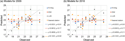
Standard image High-resolution imageThe performances of the exposure assessment models were tested with leave-one-out cross validation. The correlation between the observed and predicted values was highest in the LUR models, and negative in the nearest station models. However, the relationship was only statistically significant for the 2009 LUR model (figure 3). The station with the highest concentration in year 2009 did not perform well in all four models.
Figure 3 Plot of observed and predicted NO2 by exposure assessment methods.
Download figure:
Standard image High-resolution image
Among the exposure assessment models, the root mean square error of the LUR models was the lowest, while the nearest station model showed the highest value (table 3). The correlation between the observed and the predicted values was re-examined after excluding the two highest and three lowest stations, but the highest correlation among the four exposure models in each year remained unchanged.
Table 3. Cross-validation results: root mean square error (ppb) by exposure assessment models.
| Exposure assessment model | 2009 | 2010 |
|---|---|---|
| Kriging | 2.9 | 2.8 |
| IDW | 2.9 | 2.7 |
| LUR | 1.3 | 2.6 |
| Nearest station | 3.5 | 3.2 |
3.3. Estimation and comparison of exposure levels of the subjects in a cohort
Empirical estimates were derived for the Ulsan cohort in 2009 with the four 2009 exposure models generated in the current study. The exposure levels of NO2 for the 969 participants estimated with LUR showed the widest range (11.3–28 ppb) compared to other exposure methods, while the estimates by other exposure assessment methods were in the range of 17.7–27.9 ppb. NO2 estimated with LUR had the smallest mean (17.5 ppb) and highest variance (2.7 ppb). Similar trends were observed in 2010 (table 4).
All exposure estimates of NO2 were positively correlated across exposure methods. Especially, ordinary kriging IDW, and nearest station produced highly correlated estimates. However, the estimates by LUR were not significantly correlated with the exposure estimated produced with the nearest station method (table 5).
Table 4. Descriptive statistics of personal NO2 concentrations (ppb) of the Ulsan cohort estimated with four exposure assessment methods.
| Statistics | 2009 | 2010 | ||||||
|---|---|---|---|---|---|---|---|---|
| LUR | Kriging | IDW | Nearest station | LUR | Kriging | IDW | Nearest station | |
| Mean | 17.5 | 22.7 | 23.1 | 22.8 | 18.9 | 23.0 | 23.3 | 23.0 |
| SD | 2.7 | 1.7 | 1.1 | 2.6 | 2.0 | 1.6 | 1.0 | 2.5 |
| Min | 11.3 | 17.8 | 18.2 | 17.7 | 13.5 | 18.9 | 19.5 | 18.6 |
| Max | 28.0 | 27.5 | 26.9 | 27.9 | 26.3 | 27.7 | 27.0 | 27.9 |
| Variable | Category | N | 2009 LUR | 2010 LUR | ||
|---|---|---|---|---|---|---|
| Mean | Sd | Mean | Sd | |||
| Age | Unknown | 3 | 19.3 | 1.0 | 20.1 | 0.4 |
| <20 years | 480 | 16.8 | 2.1 | 18.5 | 1.7 | |
| 20 to 59 | 417 | 18.2 | 3.1 | 19.4 | 2.2 | |
| >60 | 69 | 18.1 | 2.8 | 19.3 | 2.0 | |
| Gender | Male | 350 | 17.4 | 2.7 | 18.9 | 2.0 |
| Female | 619 | 17.5 | 2.7 | 19.0 | 2.0 | |
| Municipality | Joong-gu | 103 | 17.5 | 2.2 | 19.0 | 1.8 |
| Nam-gu | 85 | 18.1 | 2.0 | 19.6 | 1.4 | |
| Book-gu | 230 | 17.0 | 3.2 | 18.3 | 2.5 | |
| Dong-gu | 57 | 15.4 | 3.1 | 17.2 | 2.4 | |
| Ulju-goon | 103 | 17.5 | 2.2 | 19.0 | 1.8 | |
Table 5. Correlation coefficients (p-value) between NO2 estimates in the Ulsan cohort (N = 969) by exposure method.
| Year | Method | Kriging | IDW | Nearest station |
|---|---|---|---|---|
| 2009 | LUR | 0.16 (<.0001) | 0.14 (<.0001) | 0.047 (0.14) |
| Kriging | 0.95 (<.0001) | 0.91 (<.0001) | ||
| IDW | 0.88 (<.0001) | |||
| 2010 | LUR | 0.13 (<.0001) | 0.13 (<.0001) | 0.061 (0.057) |
| Kriging | 0.97 (<.0001) | 0.91 (<.0001) | ||
| IDW | 0.88 (<.0001) |
The exposure levels of the study participants by LUR differed by demographic characteristics, especially with regard to age and region of residence (tables 4 and 6). However, the average concentrations of NO2 were all below the national annual standards of the Republic of Korea, which is 30 ppb.
4. Discussion
In this study, LUR models were built to predict the ambient NO2 concentrations of Ulsan, and the exposure estimates of the Ulsan cohort participants generated by the LUR models were compared to that of other conventionally used exposure assessment methods (i.e. nearest station, IDW, kriging). The LUR model predicting the ambient NO2 concentrations of Ulsan consisted of the area of transportation within 750 m, inverse distance to residential area, and area of wetland within 750 m. The LUR model showed high predictability and validity compared to the other three conventionally used exposure assessment models. Street-level residential addresses of the study population were used to estimate personal exposure level with the models. The empirical NO2 estimates of the Ulsan cohort by the LUR model were positively correlated with the estimates by other exposure assessment methods. The exposure levels of individuals differed by demographic characteristics. The average concentrations were below the national annual guideline for NO2 in the Republic of Korea.
The LUR model developed in the current study showed high predictability. In the LUR model, ambient NO2 increased as transportation within 750 m increased. Such a relationship is consistent with previous literature (Beelen et al 2013, Hoek et al 2008), and could be explained by the fact that traffic is a major source of NO2. Ambient NO2 was negatively associated with inverse distance to residential area. This implies that NO2 concentration increases the closer the distance is to a residential area. A positive relationship between NO2 and residential area was observed in previous literature (Beelen et al 2013), and could be explained by the air pollution emitted from residential areas. The ambient concentrations of NO2 decreased as the area of wetland within 750 m increased. An increase in the area of wetland within 750 m may be related to a decrease in pollution sources.
The 2009 LUR model explained 86% of the variation. However, there was a considerable decrease in the adjusted R2 to 45% in the calibrated 2010 LUR model. The lower predictability of the calibrated model observed may be caused by limitations in the stability of the LUR model developed in 2009, and limitations in the performances of the calibration technique applied in the current study. The stability of the LUR model may be enhanced by increasing the number of monitoring stations (Basagaña et al 2012) and obtaining additional geographical (e.g. traffic density) or temporally varying data (e.g. meteorological factors) (Liu et al 2015). The performance of the calibrated model may be hindered by the lack of temporality in LUR models (Johnson et al 2013). There have been attempts to account for temporality in LUR models, which include developing a new model with updated land-use variables (Slama et al 2007), adjusting the coefficients of the developed LUR model (Mölter et al 2010, Wang et al 2013), or applying a calibration factor of daily (Dons et al 2014, Johnson et al 2013) or seasonal variation (Slama et al 2007). The current study adjusted the coefficients of the developed LUR model, which was reported as the best performing methodology in a previous study (Wang et al 2013). Such methodology may have the underlying assumption that the types of land-use characteristics, which are associated with ambient air pollution concentrations of a certain region, are not affected by temporality. Rather, it is assumed that the strength and extent of the association between the land-use characteristics and ambient air pollution concentrations may be altered in time. Complications may arise when the underlying assumptions are violated. Further studies accounting for temporality in LUR models need to be developed. Other means of taking temporality into account are being introduced (Liu et al 2015), and warrant further attention.
In comparing the performances of the four exposure models, the LUR model showed the best performance, followed by kriging, IDW, and nearest station. The outperformance of kriging over IDW and nearest station is concordant with some previous studies, where kriging and IDW were compared using simulated data (Zimmerman et al 1999) and real data (Iñiguez et al 2009, Rivera-González et al 2015). However, the debate is ongoing about which interpolation method performs better between kriging and IDW (Cressie 1993, Hannam et al 2013). In general, kriging is considered to have better predictability compared to IDW as the sampling density increases (Wu et al 2006). The outperformance of the LUR model over other methods observed in the current study is in concordance with a previous study (Meng et al 2015). In the current study, the performance of the LUR model was comparatively high, while the performance of other methods tended to be lower. Previous literature showed that the LUR model explained 50%–90% of the variation in concentrations at sampling sites (Hoek et al 2008), while IDW and kriging explained up to 67% (Hart et al 2009) and 64% (Beelen et al 2009), respectively. A possible explanation is that the characteristics of the sampling sites in the current study may not fully represent the study area. Only 13 sampling sites were used in the current study. The 13 sites are not evenly distributed and are concentrated in the central regions of Ulsan. The distribution and number of sampling sites may be a substantial limiting factor for nearest station, IDW, and kriging methods, especially because these exposure modeling methods estimate exposure of a site based on the values nearby. The approach used to compare the predictability of four exposure assessment methods in the current study is rather simplified in a practical sense. Applying simplified measures made possible the comparison using readily-usable government-collected stationary data. However, further studies applying simulations are needed to confirm the findings.
The cross validation results of each exposure model showed that LUR models had the highest validity. In previous studies on the development of LUR models, most of the studies concentrated on building an LUR model with high internal validity and only a few studies compared the validity of the developed LUR model with other exposure models. In previous studies examining the difference in effect estimates by multiple exposure assessment methods, similar results have been observed (Hannam et al 2013, Montagne et al 2013, Meng et al 2015). However, a previous study in Canada reported that indoor and outdoor NO2 showed high correlation with personal exposure, while LUR-modeled NO2 did not, despite its high correlation with outdoor traffic-related exposure (Sahsuvaroglu et al 2009). Therefore, further studies comparing the validity and exposure estimates by multiple exposure assessment methods need to be conducted as no consensus on the comparability of exposure assessment methods exists.
The LUR modeling holds several limitations in addition to the previously mentioned benefits. The performance of LUR modeling is largely influenced by the quality and number of input land-use variables. Also, similar to conventional methods, the number and geographical distribution of exposure monitors affect LUR model performance. In previous LUR studies, air pollution information from 25–100 monitoring stations was typically employed and 40–80 were recommended (Basagaña et al 2012, Beelen et al 2013, Hoek et al 2008). Taking temporality into LUR models is another challenge, and multiple methods are being explored (Slama et al 2007, Mölter et al 2010, Wang et al 2013, Johnson et al 2013, Dons et al 2014, Liu et al 2015). Also, further improvement is needed in applying the outdoor air quality generated by LUR models to predict personal exposure (Sahsuvaroglu et al 2009).
The high performance and validity of the LUR model implies the need for further study in Asian countries. Although an increasing number of LUR studies is being conducted in Asian countries, most are limited to China (Chen et al 2010, Chen et al 2012, Li et al 2015, Liu et al 2015) and only a few applied LUR to disentangle the effects of air pollution on adverse health effects (Yorifuji et al 2010). Most of the LUR models showed low predictability ranging from 44%–64%, with only one study (Chen et al 2012) showing predictability (89%) similar to the model in the current study (86%). Two previous studies had a small number of monitors (Chen et al 2010, Chen et al 2012), and all studies performed hold-out validation rather than leave-one-out cross-validation. One of the major reasons for the limited number of studies conducted in other Asian countries may be limited knowledge of the LUR modeling itself and data availability. The current study demonstrates the implementation of LUR modeling in the Republic of Korea. Also, the small number of monitoring sites in a small industrial region with limited data in the current study could resemble settings more similar to Asian countries than European countries. Although a large number of input LUR variables may be required to build a well-performing model, various variables can be generated once land-use information is obtained via governmental databases or normalized difference vegetation index. It can be argued that the comparatively high performance of LUR over other methods may be due to more information employed to generate the model. However, generating LUR models would be of merit when comparing the trade-offs between the high-performance and the work-load given the simplicity in data acquisition, data handling, and model generating. Therefore, the authors suggest the need to explore LUR research in Asian countries.
The exposure estimated with LUR had wider ranges than estimates from the other three exposure methods, which is consistent with a previous study (Lee et al 2014). Exposure estimates of NO2 by all four exposure assessment methods were positively correlated. In particular, the estimates by kriging, IDW, and nearest station showed high positive correlations, which is in concordance with previous literature (Brauer et al 2008, Rivera-González et al 2015). However, the exposure estimated with LUR and other methods were weakly correlated, which is lower than what was observed in previous studies (Brauer et al 2008, Wang et al 2013). In particular, the estimates by LUR were not significantly associated with the estimates by the nearest-station method. A possible explanation for the low correlation observed between the estimates by LUR and other models in the current study could be that the nearest station, kriging, and IDW methods perform estimation within the range of the known values, while LUR does not restrict the boundary for the estimation process. Limitations in the monitoring stations used for analysis may have caused low performance of the nearest station, IDW, and kriging methods, resulting in low correlation with LUR. Another possibility is that the cohort may have consisted of a higher proportion of people residing in low-polluted areas. The addresses of the recruited participants were not evenly spread over Ulsan; rather, they were concentrated in the central region. The limitations in predicting the lowest and highest concentrations with the nearest station, IDW, and kriging methods and the high predictability of LUR in predicting small-area variation may have led to a higher discrepancy between the LUR model and the other three models.
The 2009 exposure models were applied to generate the empirical NO2 concentrations of the participants of the Ulsan cohort. The annual NO2 concentration estimates by LUR of the residents varied by demographic characteristics and municipality of residence. Residents under 20 years of age were exposed to lower concentrations of NO2, compared to those aged 20 years and older. Residents of Dong-gu were exposed to the lowest annual concentrations of NO2,while those living in Nam-gu were exposed to the highest levels of NO2. The high levels of NO2 observed in Nam-gu may be explained by its geographical characteristics. Nam-gu is located at the center of the city, which consists of big residential areas and a number of industrial complexes, and is located at the west of another big industrial complex. There is an industrial complex located in Dong-gu as well. However, strong wind from the sea may have facilitated the dilution process as the monitoring station in Dong-gu is located a couple of miles south-east of the complex and is located at the lower end of the peninsula. Overall, the average concentrations of annual NO2 exposure levels were all below the national guidelines in the Republic of Korea (30 ppb).
The annual NO2 concentrations of the current study cohort were among the highest compared to cohorts of previous studies (table 6). The reason for such high annual concentrations observed in the current study could be that the Ulsan cohort is a cohort located in one of the largest industrial cities in the Republic of Korea. We were able to model the exposure level of the actual residential addresses and confirm that the residential exposure to NO2 in the Ulsan cohort was below the national guideline of the Republic of Korea. Instead of estimating the annual NO2 concentrations of the entire region, we estimated the annual NO2 concentrations with regard to the actual street-level residential addresses. In terms of environmental health, the air pollution exposure in the residential area may be more of a concern, compared to the area as a whole.
Table 6. Comparison of NO2 (ppb) exposure levels by cohort.
| Author (year) | City, Country | Cohort | Population | Average | Min | Max | Exposure assessment |
|---|---|---|---|---|---|---|---|
| Aguilera et al (2007) |
Sabadell, Spain | INMA study | Pregnant women | 18.2 | 9.1 | 37.3 | LUR |
| Iñiguez et al (2009) |
Valencia, Spain | INMA study | Pregnant women | 17.7 | 3.4 | 28.2 | LUR and kriging |
| Kim et al (2014) | 3 cities, Korea | MOCEH | Pregnant women | 26.3 | 13.1 | 45.1 | IDW |
| Mann et al (2010) | Fresno, USA | FACES | Children | 18.6 |
4.6 | 52.4 | Central site |
| Gehring et al (2013) |
Germany, Sweden, Netherlands, UK | BAMSE, GINIplus, LISAplus, MAAS, PIAMA | Children | 6.8 | 2.9 | 16.1 | LUR |
| 10.6 | 5.6 | 29.8 | |||||
| 11.5 | 9.6 | 30.6 | |||||
| 11.2 | 7.8 | 14.8 | |||||
| 11.3 | 4.6 | 29.0 | |||||
| Jerrett et al (2008) |
California, USA | CHS | Children | 14.6 | Direct measurement | ||
| Lenters et al (2010) |
Utrecht, Netherlands | Atherosclerosis Risk in Young Adults study | Young adults | 18.1 |
9.6 |
21.9 |
LUR |
| Young et al (2014) | USA | Sister study | Women | 4.5 |
2.8 |
Universal kriging | |
| Jerret et al (2013) | California, USA | ACS CPS-II | General | 6.0 | 1.5 | 10.7 | LUR |
| Topp et al (2004) |
Germany | INGA | General | 12.0 |
62.1 | ||
| Heinrich (2012) |
North Rhine-Westphalia, Germany | Combined cohort | Women in mid-50s | 19.0 | 9.7 | 29.2 | Nearest |
| Foraster et al (2014) |
Girona, Spain | REGICOR | 35–83 | 13.0 |
5.4 |
LUR | |
| Beelen et al (2008) |
Netherlands | NLCS | 55–69 at enrolment | 18.0 | 7.1 | 32.5 | Regression model considering regional, urban, and local component |
| Dietrich et al (2008) |
Swiss | SAPALDIA study | Adults | 11.2 | 3.4 | 24.3 | Dispersion modelling |
| Sørensen et al (2014) |
Denmark | DCH study | 50–64 at enrolment | 8.1 |
5.8 |
16.1 |
Dispersion modelling |
| Vossoughi et al (2014) |
Ruhr, Germany | SALIA | Elderly women | 15.0 | 6.4 |
Nearest station, LUR | |
| 12.7 | 4.6 |
||||||
| Current study | Ulsan, Korea | Ulsan cohort | General | 18.9 | 13.5 | 26.3 | LUR |
aOriginally expressed in ug m−3; bOrder in BAMSE, GINI South, GINI/LISA, MAAS, PIAMA; cOrder in nearest and LUR; dMedian; e5%; fIQR; gStandard deviation; h95%.
5. Conclusion
In conclusion, the LUR models showed high performance and the widest range of exposure estimates compared to the exposure methods of nearest distance, ordinary kriging, and IDW in an industrial city in the Republic of Korea, despite the small sample size and limited data. However, the performance of the LUR model declined drastically when calibrated, suggesting the need for temporal factors in the model. Results imply that LUR method may be useful in similar settings in Asian countries where the target region is small and availability of data is low. Further studies incorporating more data and regions should be conducted in Asian countries to confirm the applicability of the LUR method.
Acknowledgments
This work was financially supported by the National Research Foundation of Korea Grant (2014R1A2A1A11052556) funded by the government of the Republic of Korea (MSIP).