

Abstract
Despite progress in impact modelling, communicating and understanding the implications of climatic change projections is challenging due to inherent complexity and a cascade of uncertainty. In this letter, we present an alternative representation of global climate change projections based on shifts in 125 multivariate strata characterized by relatively homogeneous climate. These strata form climate analogues that help in the interpretation of climate change impacts. A Random Forests classifier was calculated and applied to 63 Coupled Model Intercomparison Project Phase 5 climate scenarios at 5 arcmin resolution. Results demonstrate how shifting bioclimate strata can summarize future environmental changes and form a middle ground, conveniently integrating current knowledge of climate change impact with the interpretation advantages of categorical data but with a level of detail that resembles a continuous surface at global and regional scales. Both the agreement in major change and differences between climate change projections are visually combined, facilitating the interpretation of complex uncertainty. By making the data and the classifier available we provide a climate service that helps facilitate communication and provide new insight into the consequences of climate change.
Export citation and abstract BibTeX RIS

Original content from this work may be used under the terms of the Creative Commons Attribution 3.0 licence.
Any further distribution of this work must maintain attribution to the author(s) and the title of the work, journal citation and DOI.
1. Introduction
The last decades have revealed overwhelming evidence that the world's climate is changing (Fischer and Knutti 2015, Foster and Rahmstorf 2011, IPCC 2013). Since the 1970s an increasing effort has been placed in modelling the future climate to understand the magnitude of potential change (Coumou and Robinson 2013, IPCC 2013, Manabe and Wetherald 1975, McNeall et al 2016, Yip et al 2011). General Circulation Models (GCMs) have been run for a multitude of scenarios following alternative emissions trajectories, providing a range of plausible climate change with mean global surface temperature likely to exceed 1.5 °C- or even 3 °C in some scenarios- by the end of the century (Collins et al 2013, IPCC 2013). However, it remains difficult to understand and communicate a straightforward implication of these projected changes in generic climate variables (e.g. global mean surface temperature or annual precipitation; Leary et al 2009, Saxon et al 2005, Veloz et al 2012), especially given the great spatial and temporal variation in the projections (Flato et al 2013).
Climate impacts modelling is providing an improved understanding of potential consequences of climate change at global and continental scales (e.g. Schröter et al 2005, Sitch et al 2003, Thuiller et al 2005, Zia et al 2016). For example, dynamic global vegetation models (e.g. Sitch et al 2003) help understand consequences for primary production (Kucharik et al 2000) and global carbon balances (Piao et al 2009), while species distribution models identify vulnerable species (Thuiller et al 2011) and support nature conservation (Franklin 2010). Furthermore, integrated modelling approaches combine socio-economic and climate scenarios to assess global environmental change impacts for a wide range of domains (e.g. IMAGE Team 2001, Schröter et al 2005, Wei et al 2009). Although these approaches provide insight in specific potential impacts, these more advanced models are also paired with an increased complexity that limit their applications to a limited number of climate projections and yet present a cascade of model uncertainties that complicate understanding of their results (Jones 2000, Visser et al 2000).
In this letter, we present an alternative representation of global climate change projections for 2050 based on shifts in 125 multivariate strata with a relatively homogeneous climate. The approach has similarities to earlier global work on biomes (Leemans et al 1996, Tchebakova et al 1993), and regional studies in US (Saxon et al 2005, Veloz et al 2012) and Europe (Metzger et al 2008), but is based on the recent Global Environmental Stratification (GEnS; Metzger et al 2013b). The approach provides a convenient statistical summary of a climate change scenario by quantifying shifts in strata identifying climatic analogues (see Hallegatte et al 2007, Veloz et al 2012) that help illustrate and understand the magnitude of the projected change (e.g. desert climates from Africa moving into Spain). Such an approach can support a variety of impacts studies including crop modelling (e.g. Ewert et al 2005, Hermans et al 2010), biodiversity modelling (e.g. Verboom et al 2007), and land use change modelling (Zomer et al 2014a, 2014b). All data and algorithms are available through the University of Edinburgh data repository DataShare (Metzger et al 2017).
2. Data sources
2.1. The global environmental stratification
The construction of the Global Environmental Stratification, described in detail by Metzger et al (2013b) is based on statistical clustering to ensure that subjective choices are explicit, their implications are understood and the strata can be seen in the global context (Metzger et al 2005). Statistical screening of 42 gridded bioclimate variables derived from the WorldClim database (Hijmans et al 2005) for baseline (1960−2000) produced a subset of four variables: the annual sum of daily temperatures above 0 °C; an annual aridity index (AI) (Trabucco et al 2008); temperature seasonality; and potential evapotranspiration seasonality. These were compacted in uncorrelated dimensions using principal components analysis. Statistical clustering was subsequently used to classify the principal bioclimate gradients in temperature, aridity and seasonality into relatively similar biophysical environments. To provide structure and support a consistent nomenclature these strata were aggregated into global environmental zones based on the attribute distances between strata. The GEnS delineates 125 strata for current conditions (1961−2000), which have been aggregated into 18 global environmental zones and have a 30 arcsec resolution (approximately 1 × 1 km at the equator). The zones are displayed on the global map in figure 1(a). The zones and their containing strata are listed in table 1 with bioclimate summary statistics, which is used as a reference in the sections to follow. Added value of the GEnS compared to existing global classifications include the rigorous statistical methods used to delineate the strata, the high spatial resolution which allows for the identification of regional gradients, and the increased number of strata (e.g. in major mountain systems where altitudinal gradients are subdivided). Comparison with existing global, continental, and national stratifications confirms that it successfully partitions important environmental gradients (Metzger et al 2013b, van Wart et al 2013).

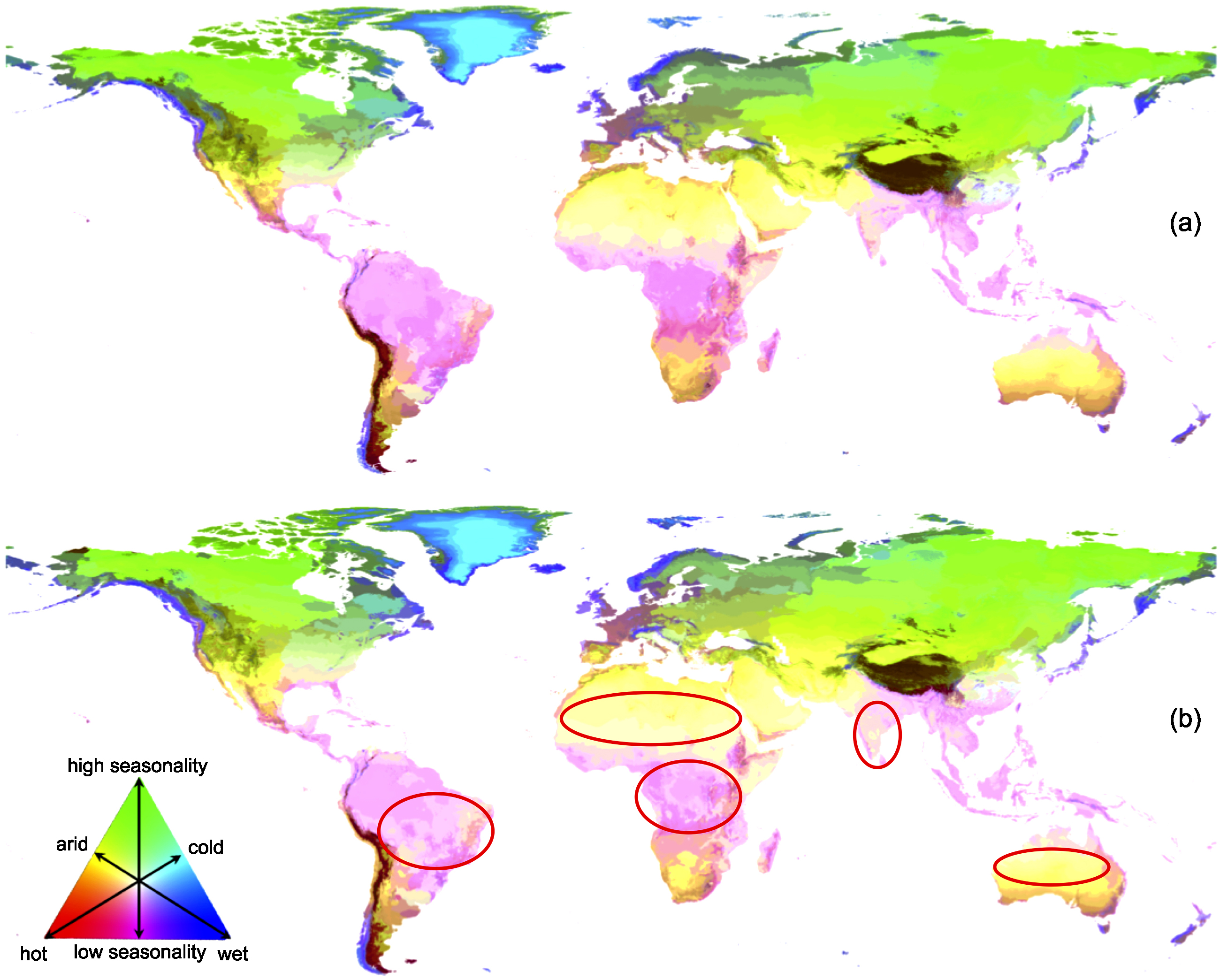
Figure 1 Distribution of the 18 environmental zones on the global map under (a) baseline and (b) future (2050, as average of 2041–2060) conditions (composite map of the 63 scenarios). The circled areas in (b) identify regions with notable zone shifts: tropical (pink) areas in South America, Africa and India become warmer and drier and shift to lighter shades. Similarly, shades of yellow in Australia and Africa are lighter indicating that these areas are becoming hotter and more arid.
Download figure:
Standard image High-resolution image2.2. WorldClim Climate change scenarios
To ensure consistency with the GEnS climate predictors, monthly climate averages from the WorldClim future climate scenarios (Hijmans et al 2005, Ramirez and Jarvis 2010) were used for the analysis to reconstruct the GEnS bioclimate variables representative for for 2050 (i.e. average over 2041–2060). These datasets were developed by downscaling a suite of 19 GCMs projections, provided by Phase 5 of the Coupled Model Intercomparison Project (CIMP5; Meehl and Bony 2011), and four Representative Concentration Pathways (RCPs; Vuuren et al 2011) emissions scenarios to 30 arcsec resolution, as described by Ramirez and Jarvis (2010). The four main RCPs were taken into consideration (i.e. RCP 2.6, RCP 4.5, RCP 6 and RCP 8.5), representing increased greenhouse gas concentrations, and thus radiative forcing. The resulting ensemble of GCMs/RCPs projections accounted for 63 elements, which represent convergence and agreement (i.e. uncertainty) among different future climate projections. Such downscaling was carried out using the Delta method, a statistical downscaling technique, which is based on the interpolation of future simulated GCM monthly climate anomalies with high resolution 'actual' monthly climate surface distributions from WorldClim (Ramirez and Jarvis 2010). It is assumed that the change in climate is relatively stable over space within a GCM pixel, while changes in future climate conditions (averages and seasonality) are driven at GCM pixel level by the GCMs projections. Statistical downscaling techniques have emerged to satisfy the need for interpolating regional-scale atmospheric predictor variables (e.g. area averages of precipitation and/or temperature; Wilby et al 1998) to resolutions high enough to represent trends needed for bioclimate studies, at least for lower order statistical moments, i.e. monthly averages (Sunyer et al 2012, Sunyer et al 2010). Furthermore, the simplicity of the assumptions behind the Delta method favour fast computing efficiency, allowing for downscaling of multi-GCMs ensemble at very high resolution to fully represent climate projections modelling uncertainty.
2.3. Data preparation
To facilitate computation, all datasets were re-sampled to 5 arcmin resolution. Although the experiment could have been carried out at 30 arcsec resolution, the lower computational cost made it possible to use multiple GCMs, allowing the maximum representation of uncertainties in climate change assessments (Hein et al 2009, Viner 2002). The resampling was carried out in ArcGIS version 9.3 (ESRI 2011), using the mean values for the bioclimate variables and BlockMajority for the nominal GEnS data. The data were then combined into a single data file with 2221696 rows, one for each 5 arcmin land surface grid cell, with the following attributes: the GEnS stratum, latitude, longitude, the four climate variables for the baseline, and for each of the 63 future scenarios (i.e. 19 GCMs and 4 RCPs, although not all 4 RCPs were available for each GCM).
3. Mapping global climate change through bioclimate classification
3.1. Classification
To map the future location of the GEnS strata a classification problem needs to be solved by finding a model, or classifier, that can adequately describe the GEnS strata based on the climate variables in baseline (i.e. the training dataset), to subsequently model their future distribution using the climate scenarios (as described above). The WEKA Data Mining Software in Java (Hall et al 2009, Witten et al 2011) was used to explore alternative classification algorithms (see appendix). Random Forests (Breiman 2001) showed superior performance in classifying the GEnS and was thus selected. The method uses a combination of multiple classification trees (i.e. rules for predicting a class given the values of its predictor variables) to provide more accurate classifications (Breiman 2001, Cutler et al 2007). Random Forests has a high classification accuracy (Cutler et al 2007) and has been used in other climate change-related modelling exercises (e.g. Cutler et al 2007, Prasad et al 2006, Rehfeldt et al 2012). Stratified cross-validation (Zhang et al 1999) was used to train the baseline dataset with Random Forests, a resampling technique using multiple random training and test subsamples. Exploratory comparisons between random subsets of the whole training dataset were used to determine the optimal settings for the Random Forests parameters, as described in detail in the appendix, resulting in a classifier that correctly classified 83.61% of the strata.
3.2. How do the global bioclimate zones shift?
The maps resulting from the classification show notable spatial shifts in the environmental zones between baseline and future (2050) conditions, as illustrated in figures 1(a) and (b). General observations are the significant spatial expansion of the Extremely Hot and Xeric zones (cf table 1) and the colonisation of cold mountaintops by warmer zones. These spatial shifts are examined below in greater detail.
Table 1. The 18 environmental zones, their GEnS strata and the mean zonal values for the annual sum of daily temperatures above 0 °C (Tsum), the annual aridity index (AI) (Trabucco et al 2008), and temperature seasonality (Tseason) expressed as the standard deviation of mean monthly temperature. Greater Tsum values indicate warmer climates, greater AI values wetter climates, and greater Tseason values more pronounced seasonality. Descriptors used in the naming of the environmental zones are based on temperature and aridity classes defined by Metzger et al (2013b).
| Environmental zones | GEnS strata | Tsum | AI | Tseason |
|---|---|---|---|---|
| Arctic 1 | 1, 2 | 0 | 16.70 | 0.91 |
| Arctic 2 | 3, 4, 5 | 2 | 9.60 | 0.97 |
| Extremely Cold & Wet 1 | 6, 7, 23 | 136 | 5.72 | 0.94 |
| Extremely Cold & Wet 2 | 8, 9, 10 | 151 | 2.20 | 1.11 |
| Cold & Wet | 13, 14, 24, 32, 39 | 1484 | 3.58 | 0.53 |
| Extremely Cold & Mesic | 11, 12, 15−22, 25−29 | 834 | 1.00 | 1.34 |
| Cold & Mesic | 30, 31, 33−38, 40−42, 44, 47, 48 | 1922 | 0.88 | 1.26 |
| Cool Temperate & Dry | 43, 45, 46, 50–52, 54, 56, 57 | 2862 | 0.53 | 1.09 |
| Cool Temperate & Xeric | 58, 59, 63−65, 69 | 3947 | 0.27 | 1.07 |
| Cool Temperate & Moist | 49, 53, 55, 60−62 | 3655 | 1.27 | 0.64 |
| Warm Temperate & Mesic | 66−68, 70−77, 80, 81 | 5197 | 0.79 | 0.65 |
| Warm Temperate & Xeric | 78, 79, 82, 84, 86, 89 | 6161 | 0.26 | 0.59 |
| Hot & Mesic | 95, 98, 100−102, 104−106 | 8213 | 0.85 | 0.23 |
| Hot & Dry | 83, 85, 87, 88, 90−94, 96, 97 | 7118 | 0.55 | 0.46 |
| Hot & Arid | 99, 103, 107 | 8149 | 0.06 | 0.68 |
| Extremely Hot & Arid | 110, 116 | 9155 | 0.08 | 0.61 |
| Extremely Hot & Xeric | 119, 121−125 | 10035 | 0.28 | 0.34 |
| Extremely Hot & Moist | 108, 109, 111−115, 117, 118, 120 | 9326 | 1.13 | 0.12 |
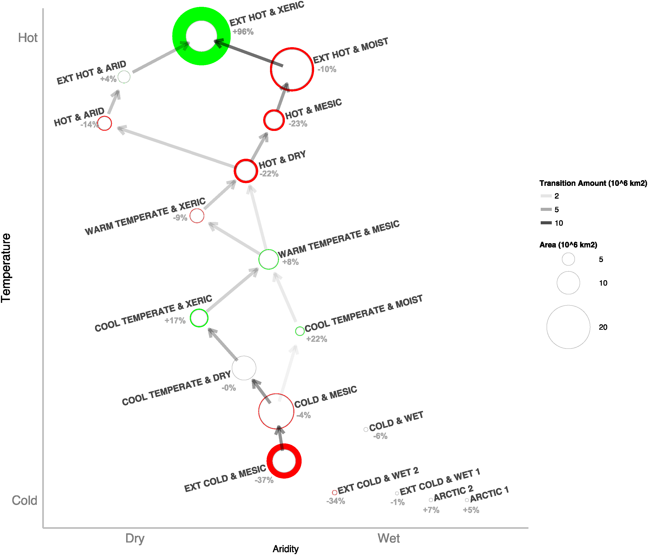
The zonal flow diagram in figure 2 shows that warmer environments generally replace cooler ones. Hot zones move towards becoming Extremely Hot & Xeric, consequently leading to a near doubling of the latter (+96% on average over the 63 scenarios). Likewise, a great decrease in the tundra-type Extremely Cold & Mesic zone (−37%) is observed, largely shifting to warmer, drier, and more temperate zones (Cool Temperate & Dry; Cool Temperate & Moist). Areas with Warm Temperate & Mesic, and with Cool Temperate & Xeric, zones are expected to increase, replacing colder zones. In figure 3 we observe that zones generally shift poleward. The Arctic is invaded by wetter zones ([Extremely] Cold & Mesic; [Extremely] Cold & Wet). Areas between the Tropic of Cancer and the Tropic of Capricorn are becoming warmer. Warm Temperate environments are becoming less mesic and more xeric. Notable areas that do not experience shift are the Extremely Hot & Xeric zone, parts of the tropic Extremely Hot & Moist zone, the coldest areas of the polar regions, and some wet oceanic regions (see supplementary data stacks.iop.org/ERL/12/084002/mmedia).

Figure 2 Zonal flow diagram, showing both the areal transitions between zones and the overall and relative changes in area averaged over all 63 GCMs for the 2050 time-slice. Transition amount is calculated by comparing the starting and ending class of each grid cell and by aggregating. It is represented by the intensity of arrows between each zone (transitions with less than 50000 km2 are removed). Areal change is calculated by comparing the total area of each class to the baseline value. Each class is represented by a circle which is coloured according to whether area increases (green) or decreases (red). Spatial structure is provided by aridity and temperature, with each class centred on its baseline average. This figure was produced in R (R Core Team 2015).
Download figure:
Standard image High-resolution image
Figure 3 Violin plot of the environmental zones' latitudinal distribution. The violin lines represent the distribution of each zone against latitude, normalized so that each violin has full width. Future distributions come from a random sample of 4 million points from all 63 scenarios. Individual points are plotted to indicate the absolute density of each zone as well. Note that in many cases, the long tail of each violin towards the equator is due to small mountainous regions near the equator. The general trend is for zones to shift more toward the poles. Examples include the shift in density in the Cold & Mesic, Cool Temperate & Dry and Extremely Cold & Mesic zones towards more northern latitudes. This figure was produced in R (R Core Team 2015).
Download figure:
Standard image High-resolution image3.3. What do shifts look like at a regional scale?
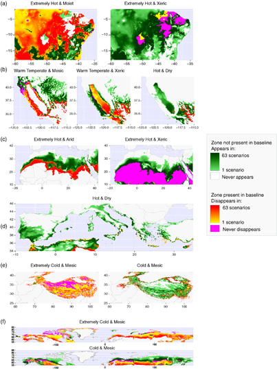
It is not possible to provide an extensive range of regional examples in this letter, but we provide several noteworthy examples that illustrate how the shifts of individual environmental zones and GEnS strata provide a convenient and informative summary of global and regional environmental change. The examples were selected to demonstrate climate change impacts on, among others, major agricultural regions, deserts, mountain ranges, permafrost environments and tundra biomes (figure 4).
Figure 4 Examples of notable shifts of different environmental zones. The legend indicates how many of the 63 climate scenarios appear (green), disappear (orange), and remain stable (pink). Comparing maps for different zones provides insight how zones are replaced. The colour gradients reveal the number of scenarios indicating a shift, and therefore provides an indication of the likelihood or uncertainty of change. (a) Cerrado, Brazil, where existing Extremely Hot & Xeric zone persists and replaces Extremely Hot & Moist; (b) California, USA, where zone Warm Temperate & Xeric replaces Warm Temperate & Mesic, and is in turn replaced with Hot & Dry; (c) Sahara, Africa where Extremely Hot & Arid zone spreads northwards and is replaced by Extremely Hot & Xeric; (d) the Mediterranean, showing the expansion of zone Hot & Dry; (e) the Himalayas where extremely cold areas are warming (from zone Extremely Cold & Mesic to Cold & Mesic); and (f) the Northern Hemisphere, again showing a warming effect as in (e). This figure was produced in R (R Core Team 2015).
Download figure:
Standard image High-resolution image
At a regional scale, the shifts in strata illustrate that major agricultural regions becoming hotter and drier. For example, the Cerrado in Brazil shifts from Extremely Hot & Moist to Extremely Hot & Xeric (figure 4(a)), with strata 122 and 123 expanding greatly in the region (supplementary data); and in California, USA, shifts from Warm Temperate & Mesic to Warm Temperate & Xeric (figure 4(b)) and Hot & Dry (especially strata 78, 82, 84, 86, 89, 91, 92 and 96; supplementary data).
The expansion of desert-like climates is clearly visible in the maps. For example, the Sahara shows a northward expansion of the Extremely Hot & Xeric zone in (strata 119, 121, 124 and 125; supplementary data), replacing zone Extremely Hot & Arid, which also shifts northward (figures 4(c) and (d)). Meanwhile, the Mediterranean countries Spain, Portugal, Italy, Greece and Cyprus are occupied by zone Hot & Dry, currently prevalent in the north of Africa (figure 4(d)).
Conversely, the maps illustrate the extent to which colder climes contract. For example, in the Himalayas zone Extremely Cold & Mesic is largely replaced by the warmer zone Cold & Mesic (figure 4(e); strata 37 and 42; supplementary data). Similarly, permafrost environments and tundra biomes show a great decline. Zone Extremely Cold & Mesic in the Northern Hemisphere is replaced by the warmer zone Cold & Mesic (figure 4(f); strata 30, 31, 34, 35, 36, 40, 41, 44 and 48; supplementary data).
4. Discussion
The examples above demonstrate how shifting bioclimate strata summarize future environmental shifts at global and regional scales. Both the agreement in major change and differences between climate change projections are visually combined (figures 1–4), facilitating the interpretation of complex uncertainty. The data reported here present a major advance over earlier attempts at mapping bioclimate shifts (e.g Alessandri et al 2014, Beck et al 2005, Belda et al 2016, Jylhä et al 2010, Leemans et al 1996, Mahlstein et al 2013, Metzger et al 2008, Rohli et al 2015, Saxon et al 2005, Wang and Overland 2004) due to its greater thematic resolution (125 strata) and spatial resolution (5 arcmin). Its global coverage also provides consistency for comparative analyses, and provides the potential for the dataset to be used as a consistent tool for global assessments. Zomer et al have already demonstrated how the GEnS can be used to understand potential vegetation change in the Himalayas (2014b), and climate change impacts on biodiversity and rubber production in Yunnan, China (2014a).
The most notable methodological limitation is the fact that the strata are fixed on the current climate. It does not allow for the emergence of hotter and drier strata in the future, i.e. the hottest parts of the Sahara will always remain in the Extremely Hot & Xeric stratum 125. Furthermore, novel climates with annual profiles that do not currently exist will not be identified as such, but assigned to the most similar current climate. These issues are inherent in any approach using climate analogues (e.g. Hallegatte et al 2007, Veloz et al 2012) to understand change.
The efficiency of the Random Forests classifier (appendix) was important to be able to run analyses on desktop computers. Although 16% of grid cells were misclassified due to heterogeneity within the strata, these cells would have been assigned to strata that are climatically similar (Metzger et al 2008), and consequently any interpretation errors will be small. The classifier is freely available (Metzger et al 2017), and can be used to map the GEnS strata for future WorldClim climate change projections, as well as for the 30 arcsec (approximately 1 km2) data. The latter proved too detailed for global calculations, but provide valuable detail in regional applications (cf Zomer et al 2014a, 2014b).
5. Conclusion
The bioclimate shifts presented here form a middle ground, conveniently summarizing current knowledge of climate change with the interpretation advantages of categorical data but a level of detail that resembles a continuous surface. By making the shifting GEnS datasets and the classifier available (Metzger et al 2017) we provide a climate service that helps facilitate communication and provide new insight into the consequences of climate change.
Appendix. Methods for calculating strata shifts
1. Training the classifiers
1.1. Classifier selection
Alternative models, or classifiers, for mapping the location of the GEnS strata were explored in the WEKA Data Mining Software in Java (Hall et al 2009, Witten et al 2011), version 3–6–4. Two algorithms were deemed especially promising: a decision tree (Random Forests; Breiman 2001) and a Bayesian classifier (Naïve Bayes; John and Langley 1995). Random Forests comprises a combination of classification trees to provide more accurate classifications (Breiman 2001, Cutler et al 2007) and is considered an effective tool in prediction (Breiman 2001) due to its high classification accuracy (Cutler et al 2007). Naïve Bayes is based on Bayes' rule of conditional probability and the algorithm operates under the simplistic assumptions that attributes in a given dataset are independent, and follow the normal (Gaussian) probability distribution (Witten et al 2011). Despite these simplistic assumptions, it is generally agreed that Naïve Bayes is highly effective when tested on actual datasets (e.g. Friedman et al 1997, John and Langley 1995, Turhan and Bener 2009, Vaidya 2008).
Stratified multiple-fold cross-validation was used to train the baseline dataset with the two algorithms, by resampling multiple random training and test subsamples (Zhang et al 1999). Specifically, it creates a sub-set of the dataset (training set) for each fold that is then trained on the remaining data (test set) to test the algorithm's ability to predict the actual dataset. The method has the advantage over other training methods (e.g. data splitting into training and test sets) that all observations of the datasets can be used for training and testing the model, thus reducing any uneven representation in training and test sets (Witten et al 2011, Zhang et al 1999). Ten folds were used as this is the recommended number of folds to get the best error estimate from the cross-validation technique (e.g. Borra and Di Ciaccio 2010, Kim 2009, Li et al 2010, Witten et al 2011).
Given the substantial size of the baseline dataset (2221696 rows by 4 bioclimatic variables + 125 GEnS strata), the optimal parameter settings for the Random Forests algorithm (i.e. the number of trees selected, their maximum depth and the number of attributes used in the random selection) were determined using a subset of the data. A stratified 3% random sample without replacement was used as the training set to obtain an estimate of the classifier's performance for different combinations of parameter values, a common method in data mining to save computing time (Borra and Di Ciaccio 2010). This exercise revealed that: (1) infinite maximum tree depth significantly increased calculation time and model size without necessarily improving the classifier's accuracy; (2) selecting more than 16 trees gave negligible changes in the classifier's accuracy despite increasing computing time; (3) classification accuracy stabilized around 82% when maximum depth ranged from 10−15 and number of trees ranged from 10–25 The final parameter settings were chosen following further training experiments with stratified 5%, 7%, 14% and 25% random samples without replacement of the baseline dataset (i.e. selecting three random features and ten trees with a maximum depth of 11 for each tree), which were then used to run the entire baseline dataset resulting in a 29 Mb model that could correctly predict 83.61% of the grid cells.
Conversely, Naïve Bayes is a very simple classifier with fixed parameters, making it possible to use the whole baseline dataset for training without initial testing. Naive Bayes' simplicity allowed for a fast training time (approximately 40 min) on the whole baseline dataset, correctly classifying 78.31% of the strata using a 44 Kb model. Although the classification accuracy was only slightly lower than for Random Forests, there were significant misclassifications of certain strata. Further inspection revealed strata with relatively large variation to points in the extremes of the distribution. Others have previously noted that Naïve Bayes is best suited for smaller datasets, an opinion supported by various studies (e.g. Catal and Diri 2009, Chandra and Gupta 2011).
Based on this analysis the Random Forests classifier was chosen for further analysis of the shifting strata.
Acknowledgments
The authors would like to thank the two anonymous reviewers for their constructive feedback and suggestions. ADS would like to thank Dr Eibe Frank from The University of Waikato for his invaluable support with the WEKA software. ADS gratefully acknowledges support from the A.G. Leventis Foundation (personal grant) and The University of Edinburgh MSc Integrated Resource Management (publication bursary). MJM would like to acknowledge support from the European Commission Seventh Framework Programme under Grant Agreement No. FP7-ENV-2012-308393-2 (OPERAs).