

Abstract
Unprecedented decreases in atmospheric nitrogen (N) deposition together with increases in agricultural N-use efficiency have led to decreases in net anthropogenic N inputs in many eastern US and Canadian watersheds as well as in Europe. Despite such decreases, N concentrations in streams and rivers continue to increase, and problems of coastal eutrophication remain acute. Such a mismatch between N inputs and outputs can arise due to legacy N accumulation and subsequent lag times between implementation of conservation measures and improvements in water quality. In the present study, we quantified such lag times by pairing long-term N input trajectories with stream nitrate concentration data for 16 nested subwatersheds in a 6800 km2, Southern Ontario watershed. Our results show significant nonlinearity between N inputs and outputs, with a strong hysteresis effect indicative of decadal-scale lag times. The mean annual lag time was found to be 24.5 years, with lags varying seasonally, likely due to differences in N-delivery pathways. Lag times were found to be negatively correlated with both tile drainage and watershed slope, with tile drainage being a dominant control in fall and watershed slope being significant during the spring snowmelt period. Quantification of such lags will be crucial to policy-makers as they struggle to set appropriate goals for water quality improvement in human-impacted watersheds.
Export citation and abstract BibTeX RIS

Original content from this work may be used under the terms of the Creative Commons Attribution 3.0 licence.
Any further distribution of this work must maintain attribution to the author(s) and the title of the work, journal citation and DOI.
1. Introduction
Nutrient-driven hypoxia is a continuing problem in near-coastal waters around the world, from the South China Sea in Asia [1] to the Baltic Sea in Europe [2] and the Gulf of Mexico [3] in North America. Freshwater lakes also continue to be plagued by problems of eutrophication, with excess nutrient loading leading to reports of harmful cyanobacterial blooms in areas such as Lake Taihu in China and Lake Erie in North America [4, 5]. Such nutrient enrichment poses a threat to drinking water quality and can disrupt the biogeochemical and ecological stability of freshwater and saltwater habitats.
For decades, attempts have been made to reduce the discharge of nutrients to surface and groundwater, from the upgrading of wastewater treatment plants (WWTPs) to implementation of agricultural best management practices, including reduction of nitrogen (N) and phosphorus (P) application rates, construction of treatment wetlands, utilization of controlled drainage, and the creation of riparian buffer zones [6, 7]. In some areas, changes in atmospheric emissions policies have also significantly reduced N inputs to the landscape [8]. For example, in the US and Canada, successful emission controls and more stringent vehicle standards [9, 10] together with climate-related changes in prevailing air-mass trajectories [8] have led to approximately 50% decreases in NOx deposition across the eastern states and provinces.
Despite such changes, there has been limited progress in achieving nutrient water quality goals [11]. In the Netherlands, for example, a phased program to meet water quality goals for N and P was implemented in 1985 [12]; more than 20 years later, however, only 25% of surface waters in the Netherlands met the established standards for N and P [13]. In North America, ambitious goals were set in the 1980s to reduce 'controllable' N and P loading to the Chesapeake Bay by 40%, and in 2008 the Mississippi River/Gulf of Mexico Waters Nutrient task force set the goal of reducing the size of the summer hypoxic zone to 5000 km2 by 2015 [14, 15]. In neither of these cases have nutrient goals been achieved, and target dates have now been extended by up to two decades [14, 16].
Numerous obstacles can prevent the achievement of water quality goals, including limited funding, lags in implementation of conservation measures, and a lack of knowledge regarding appropriate interventions [11, 17]. However, even with appropriate and timely implementation of best management practices, it is increasingly accepted that nutrient legacies, resulting from decades of fertilizer application and intensive livestock production, can lead to time lags in catchment-scale nutrient delivery, thus significantly delaying the achievement of measurable changes in water quality [11, 18–20]. Such time lags can occur via a range of mechanisms, from temporary storage of nutrients in soil or vegetation [21], to long hydrologic transport times through the subsurface, to retention of nutrients in stream sediments and surface water reservoirs [22]. It is now well understood that, for N, hydrologic delays due to slow groundwater travel pathways may result in very slow improvements in water quality [18, 19], and a growing body of work is focusing on quantification of hydrologic transit times through the subsurface [23–26]. It is also being recognized that while slow groundwater transit times lead to hydrologic lags, N retention in both soils and sediments can lead to additional biogeochemical time lags that are relatively less studied and more complex to quantify [18, 20, 27].
Long time lags to achieving improvements in water quality can lead to disillusionment among stakeholders regarding the potential for achieving meaningful changes in water quality. Such lags can also lead unnecessarily to calls for investment in more drastic mitigation strategies. In 2010, for example, the European Environmental Bureau stated that 'time lags' were simply a 'generic excuse' generated to avoid implementation of more stringent policy measures [28, 29]. Even among the scientific community, where the existence of nutrient-related time lags is more accepted, we continue to lack appropriate techniques for quantifying these lags, particularly techniques that can account for the diversity of landscape and management drivers that may impact the time scales over which change may occur. Although there is increasing interest in calculating long-term N and P balance trajectories [30, 31] as well as quantifying long-term trends in nutrient loading [32], there has until now been no systematic attempt to link these long-term trajectories of nutrient inputs and outputs to improve our understanding of catchment-scale time lags.
In the present study, we focus specifically on N dynamics, with the goal of quantifying N-related time lags and of identifying the primary physical and management controls on these lags. To achieve these goals, we use as a case study the Grand River watershed (GRW) in Southern Ontario, Canada, the largest watershed draining into Lake Erie. Lake Erie is one of North America's Laurentian Great Lakes, the largest freshwater system in the world, and has the highest nutrient loadings of all the Great Lakes [33]. The GRW's long history of intensive agriculture as well as its currently large urban footprint, both of which have led to significant changes in stream and groundwater nitrate concentrations over time, make the watershed an ideal candidate for analysis of catchment-scale time lags. In our exploration of GRW nutrient dynamics, we use a statistical analysis of long-term N input and output data to address the following questions:
- Can long-term N mass balance trajectories and stream N concentration data be used to quantify time lags in catchment-scale N response?
- What is the magnitude of these time lags, and do they vary according to season?
- What are the primary landscape and management controls on annual and seasonal time lags?
2. Methods
2.1. Study area
The Grand River watershed (GRW), located in southwestern Ontario, covers an area of approximately 6800 km2 and is the largest Canadian watershed draining into Lake Erie [34]. Typical of many watersheds in the eastern US and Canada, the GRW remains heavily influenced by agriculture but has also in recent decades been characterized by a loss of agricultural land, reforestation, and increasing urbanization [35]. Although agriculture is the dominant land use in the watershed, the central portion of the watershed is also home to areas of intense urbanization. Accordingly, population densities as well as the intensity of agricultural land use vary significantly across the watershed.
The surficial geology of the GRW is heterogeneous (figure 1). The watershed can be divided into three geologic zones: the upper till plain, the central gravel moraines, and the lower clay plain. The upper till plain, which encompasses both the northern and more western subwatersheds of the GRW, is characterized by low permeability and a high ratio of surface runoff to base flow [36]. In contrast, the central region of the watershed is highly permeable with high levels of groundwater recharge. Finally, the lower GRW has silt-dominated soil and very high levels of runoff. The hydrology of the GRW has been modified by both damming and tile drainage. Seven large reservoirs have been constructed on both the main stem and tributaries of the Grand, and subsurface drains (tile drainage) are heavily utilized in the upper till plain to remove excess water from cropland and route it into nearby ditches and streams (figure 1).
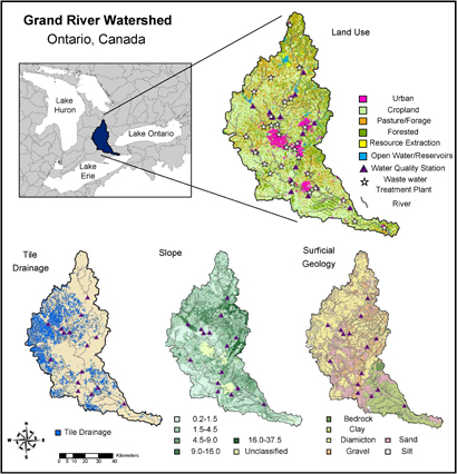
Figure 1. Grand River watershed, southern Ontario. The figure shows variations in land use, tile drainage density, slope and surficial geology across the watershed as well as the locations of wastewater treatment plants, indicated by stars. The purple triangles indicate the locations of the water quality stations used in the subwatershed analysis.
Download figure:
Standard image High-resolution imageFor our analysis, we focus on 16 subwatersheds across the GRW; of these, nine are tributaries to the Grand River and the other seven are along the river's main stem (see the supporting information (SI), section S1.1, table S1.1, available at stacks.iop.org/ERL/12/084017/mmedia).
2.2. N balance calculations
Net anthropogenic N input (NANI) trajectories were calculated for the period 1901–2011 for the GRW subwatersheds utilizing long-term NANI data calculated at the county scale. NANI values, which have been used to characterize the intensity of human perturbation of the N cycle in numerous watershed-scale studies [37–40] were calculated, with minor modification, as described by Hong et al [41]. In brief, NANI is expressed as the difference between anthropogenic N inputs (inorganic N fertilizers, animal manure, biological N fixation, atmospheric N deposition, and wastewater N) and outputs (crop N production, livestock N production). For additional details see SI, section 1.2. NANI values are reported herein as kg ha−1.
2.3. Stream nitrate trend analysis
2.3.1. Discharge and water quality data
Daily discharge data was obtained from the Water Survey of Canada.[42] N concentration data was obtained from the Ontario Provincial Water Quality Monitoring Network (PWQMN; Ontario Ministry of Environment). PWQMN monitoring stations were chosen for the current analysis based on the following criteria: (a) location with the GRW; (b) proximity to a Ministry of Environment (Canada) flow-monitoring station with temporally corresponding discharge data; and (c) available sampling data over a period of at least 25 years. The longest record length for any of the stations was 51 years (1964–2015), and 87% of stations had data available over a period of at least 35 years.
2.3.2. Estimation of flow-weighted nitrate concentrations
We used the weighted regression on time, discharge, and season (WRTDS) modeling approach [43] to estimate flow-weighted concentrations (FWCs) from intermittently measured concentration and continuously measured flow data. Daily concentration values were calculated in WRTDS via the following equation:
where, c is concentration [ML−3], β0,β1,β2,β3,β4, are fitted regression coefficients, Q [L3T−1] is daily streamflow, t [T] is time, and ε is an error term. A close 1:1 relationship was obtained between observed and predicted concentration values (mean error = −0.01 mg mg NO3-N/L), with a mean percent bias for all stations of −0.01 (SI, part I, tables S1.1 and S1.2).
Seasonal and annual FWCs were calculated from measured daily discharge and estimated daily concentrations (equation 5.4) using the following equation:
where the numerator is the annual or seasonal N load and the denominator is the total annual or seasonal discharge. Seasonal FWC values were calculated for the winter (December, January, February), spring (March, April, May), summer (June, July, August) and fall (September, October, November) seasons.
2.4. Cross correlation analysis to quantify time lags
Cross-correlation function (CCF) analysis, a statistical method for measuring correlations between two time-shifted variables, was used to quantify time lags between annual NANI and annual (or seasonal) nitrate FWCs [39, 44] (SI, section 2). FWC values, unlike non-weighted concentration values, are adjusted on the basis of variations in streamflow over a specified time period [45] and allow us to minimize the impacts of interannual variations in discharge when assessing long-term trends in N retention and N flux.
2.5. Multiple linear regression analysis to quantify dominant controls on time lags
A multiple linear regression (MLR) approach was utilized to identify dominant controls on annual and seasonal time lags for the 16 study watersheds. First, simple correlation analysis was used to identify significant relationships between both annual and seasonal time lags and a range of watershed variables. Spatial data for the analysis was obtained from the Grand River Information Network [46]. Management data, including annual NANI values, fertilizer and manure application, and population density were derived from data underlying the NANI calculations described in section 2.2. Variables showing a significant relationship (p < 0.05) with annual or seasonal lag times were considered key candidate variables for initial inclusion in the MLR analysis (SI, part III, table S3.1). Pearson correlation coefficient (r) and variance inflation factor (VIF) values were then calculated among the candidate variables [47], with r ≥ 0.80 and/or VIF ≤ 10 being considered indicative of strong collinearity (SI, part II, table S3.2). A stepwise regression approach was used to create the annual and seasonal MLR models, with systematic exclusion of highly correlated (VIF > 10) variables (O'Brien 2007). Akaike's information criterion (AIC) values were used to evaluate the resulting MLR models (Tsai et al 2007).
3. Results and discussion
The primary objectives of the present study were [1] to quantify time lags between changes in annual N inputs and subsequent changes in water quality; [2] to explore the seasonality of these lags; and [3] to identify primary landscape and management controls on both annual and seasonal lags. We describe the results of these explorations below.
3.1. Temporal trends in annual NANI values and flow-weighted nitrate concentrations
3.1.1. N mass balance trajectories
Trajectories of net anthropogenic N inputs (NANI) were developed for the period 1901–2011 for the GRW subwatersheds, as described in section 2.2. Across the GRW, annual NANI values nearly doubled, from 46 kg N ha−1 yr−1 to 87 kg N ha−1 yr−1, between 1901 and 1976, and then decreased to 72 kg N ha−1 yr−1 by 2011 (figure 2). NANI trajectories for the GRW subwatersheds show similar patterns, peaking between 1976 and 1980 and then subsequently decreasing (figure 2). The extent of that decrease has ranged from 10.5%–39.8%, with a median percent decrease of 16.5%. The decrease in N inputs can primarily be attributed to an approximately 10% decreases in atmospheric N deposition as well as increases in the N use efficiency associated with agricultural production [48].

Figure 2. Net N input trajectories for the 16 subwatersheds used in our analyses. Trajectories for the tributaries are represented by dotted lines, while those for the main stem of the Grand are represented by solid lines.
Download figure:
Standard image High-resolution image3.1.2. Nitrate concentration trajectories
Flow-weighted nitrate concentrations show an increasing temporal trend in the 1964–1992 timeframe across all the 16 subwatersheds analyzed in this paper (SI, part 4, table S4). These increases were found to be significant at a 99% confidence level (p < 0.01) for all but three of the subwatersheds. For the period 1993–2011, however, concentration trends have varied across the GRW. Only 3 of the 16 subwatersheds show a decreasing trend for nitrate FWCs over this period, while 13 continue to show an increasing trend. As a whole, the data show that nitrate FWCs increasing before 1993 at a mean rate of mg l−1 y−1; after 1993, concentrations continue to increase in the mean, but at reduced rates (mg l−1 y−1) and with a greater distribution of behavior across the different subwatersheds.
3.1.3. Hysteresis in N input-output trajectories
Spatial analysis of the GRW subwatersheds for the period 2000–2010 shows a strong linear relationship between NANI (inputs) and mean flow-weighted nitrate concentrations (outputs) (R2 = 0.64, p < 0.001). However, a look at relationships between inputs (NANI) and outputs (nitrate FWC values) over time for individual subwatersheds indicates a disruption in the linearity of the input/output relationship.
As seen in figure 3(a), annual NANI values for the Grand River at Brantford began to decrease in the late 1970s, but there has been no decrease in annual nitrate FWCs since that time, although the slope value for concentration vs time for the post-1993 period (0.022 ± 0.007 mg l−1 y−1, R2 = 0.35) has decreased somewhat from that before 1993 (0.078 ± 0.002 mg l−1 y−1, R2 = 0.98). For the Lower Canagagigue, however (figure 3(b)), the response to changes in NANI have been faster, with a peak for flow-weighted nitrate concentrations being seen in 1997 at 8.3 mg l−1, and then with significant decreases in FWC values for the post-1993 period of 0.120 ± 0.017 mg l−1 y−1.
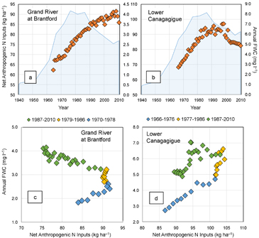
Figure 3. Temporal trajectories of annual net N inputs and annual flow-weighted nitrate concentration values from 1940–2010 for (a) the Grand River at Brantford, and (b) the Lower Canagagigue. Annual flow-weighted nitrate concentrations are indicated by the orange diamonds, and net N inputs are represented by the shaded blue area. While the N input trajectories for the two subwatersheds are similar, the concentration trajectories are quite different, with the Lower Canagagigue showing a much quicker response to changes in input values. These differences are also apparent when plotting flow-weighted concentrations against NANI, with the Lower Canagagigue (d) showing a tighter hysteresis loop than the Grand River at Brantford (c).
Download figure:
Standard image High-resolution imageThe results described above are suggestive of a mismatch between annual NANI values and annual nitrate FWCs. For example, in figure 3(c) we see a positive linear relationship between NANI values and N outputs (annual FWC) for the slower-responding main stem of the Grand up until approximately 1978 (R2 = 0.93). From 1979–1986, however, there is a period of nonlinearity during which NANI values remain relatively constant, while FWC values continue to increase. Beginning in 1987, a negative relationship develops between current-year NANI values and flow-weighted nitrate concentrations. This negative relationship between current inputs and outputs indicates a potentially lagged relationship and thus creates a visible hysteresis effect in the response curve of NANI versus nitrate concentration values. For the Lower Canagagigue (figure 3(d), the hysteresis loop is tighter than that for the Grand River at Brantford, and by 2010 shows a return to late 1970s-level nitrate FWCs. The tighter hysteresis loop for the Lower Canagagigue suggests that this smaller tributary responds more quickly to changes in N inputs than the main stem of the Grand, meaning that current nutrient dynamics in the watershed are less driven by N legacies and thus that time lags will be shorter.
3.2. Quantification of annual and seasonal time lags
3.2.1. Annual lags
The cross-correlation results provide us with estimates of time lags between changes in annual NANI values and subsequent changes in flow-weighted nitrate concentrations. Annual lag times for the 16 study watersheds were found to range from 12–34 years, with a median value of 25.5 years (SI, part 5, table S5).
Lag times were generally found to be the longest in the northern subwatersheds (30–33 years), decreasing in the middle GRW, and then increasing again in the lower GRW. The longer lag times in the northern watersheds correspond to areas of low permeability and high surface runoff, but also to areas with lower NANI values (figure 4), less cropland, higher fractions of forested area, and little tile drainage (figure 1). In contrast, the shorter lags in the middle GRW correspond to areas with more tile drainage as well as larger urban areas and their associated WWTPs. In the lower GRW, which is more dominated by groundwater flows, lag times again increase, with slow subsurface transport of nitrate via groundwater pathways likely contributing to the longer lags.

Figure 4. Spatial patterns in annual lag times across the Grand River watershed. Lag times are represented by circles, with larger circles corresponding to greater lags. The grey-scale background represents mean annual N inputs (2000–2010), which range from 28–111 kg ha−1 (darker grey corresponds to higher values). The map shows the longest lags in the upper subwatersheds and the shortest in the central portions of the basin, particularly in those subwatersheds in areas with dense tile drainage networks (see figure 1) and higher NANI values.
Download figure:
Standard image High-resolution image3.2.2. Seasonal lags
Time lags in the GRW also show seasonal variation. As an example, we show in figure 5 the monthly nitrate FWC trajectories superimposed against NANI values for the Grand River at Glen Morris Bridge. Our cross-correlation analysis of annual NANI and FWC values indicates a lag time of 20 years for this site. The monthly trajectories shown in the figure, however, show a range of behaviors across the year. In the summer, concentration values are increasing consistently over the study period, with little or no response to the decreasing post-1976 net N inputs. In the fall and winter, however, the watershed appears much more responsive to decreases in N inputs, with distinct peaks and subsequent decreases in the N concentration trajectories. In fall and winter, for example, the slope values for the pre-1993 period (0.077 ± 0.002 mg l−1 y−1, R2 = 0.98, fall; 0.105 ± 0.005 mg l−1 y−1, R2 = 0.94, winter) are significantly different from those for the post-1993 period (0.002 ± 0.006 mg l−1 y−1, R2 = 0.01, fall; 0.017 ± 0.014 mg l−1 y−1, R2 = 0.08, winter). In summer, however, the slope values for the pre- and post-1993 periods are statistically indistinguishable (0.060 ± 0.002 mg l−1 y−1, R2 = 0.98, pre-1993; 0.041 ± 0.002 mg l−1 y−1, R2 = 0.95, post-1993). Across all the subwatersheds, seasonal cross-correlation analysis indicates that median N-related time lags are the longest in summer (median 26.0; iqr = 19.8–28.5), although variability among stations is significant. In the following section, we explore the dominant controls on annual as well as seasonal time lags to further elucidate the observed spatial and temporal variability in the identified lag times.

Figure 5. Seasonal trends in seasonal flow-weighted nitrate concentrations in relation to annual net N input trajectories for the Grand River at Glenn Morris Bridge. Seasonal flow-weighted nitrate concentrations are indicated by the orange diamonds, and net N inputs are represented by the shaded blue area.
Download figure:
Standard image High-resolution image3.3. Dominant controls on annual and seasonal time lags
Based on correlation analysis of potential explanatory variables and both annual and seasonal time lags, we identified the following factors as potentially relevant for inclusion in the multiple linear regression models: percent soil organic matter (OM), fractional tile-drained area (TILE), fractional wetland area (WET), mean watershed slope (SLOPE), population density (POP), mean annual NANI values (2000–2010), and the percent cropped area (CRP). Variance inflation factor (VIF) analysis indicated strong collinearity among NANI values, fractional tile-drained area, and percent wetland area for the subwatersheds (SI, part III, table S3.2). The strong positive relationship between NANI and the percent tile-drained area (r = 0.82) can be explained by the intensive agricultural production occurring on tile-drained land, leading to higher net nitrogen inputs occurring in tile-drained areas. The strong negative relationship between tile drainage and percent wetland area (r =−0.93) is also straightforward—the installation of subsurface drainage systems results in a loss of wetland area.
In table 1 we present the set of models (p < 0.05) that best explain the annual and seasonal lag times, respectively, for the subwatersheds included in the present analysis. Complete MLR results are provided in SI, table 3.3.
Table 1. The 95% confidence set of MLR models predicting annual and seasonal lag times for the 16 study watersheds. Plus and minus signs next to the model variables indicate positive or negative correlations, respectively.
| Dependent variable | Model | Variables in the modela | R2 | p-value | AICc |
|---|---|---|---|---|---|
| Annual Lag | a6 | WET(+) | 0.28 | 0.036 | 100.1 |
| a7 | NANI(−) | 0.42 | 0.006 | 96.4 | |
| Winter Lag | w1 | CRP(+) | 0.34 | 0.022 | 102.5 |
| Spring Lag | spr5 | TILE(−), SLOPE(−) | 0.62 | 0.002 | 93.6 |
| spr6 | WET(+), SLOPE(−) | 0.61 | 0.002 | 94.0 | |
| spr7 | NANI(−), SLOPE(−) | 0.6 | 0.003 | 94.5 | |
| spr11 | SLOPE(−) | 0.34 | 0.018 | 100.4 | |
| Summer Lag | sum7 | NANI(−) | 0.54 | 0.001 | 95.6 |
| sum9 | OM(+) | 0.25 | 0.047 | 103.4 | |
| sum10 | POP(−) | 0.33 | 0.019 | 101.6 | |
| sum12 | WET(+) | 0.47 | 0.003 | 97.8 | |
| Fall Lag | f5 | TILE(−) | 0.47 | 0.005 | 99.6 |
| f6 | WET(+) | 0.43 | 0.008 | 100.8 | |
| f7 | NANI(−) | 0.46 | 0.006 | 99.9 |
aNANI=net anthropogenic N inputs, WET=percent wetland area, CRP=fractional cropped area, SLOPE=mean watershed slope, TILE=fractional tile-drained area, POP=population density, OM=percent soil organic matter. cAkaike information criterion values.
For both annual and summer time lags, the strongest, statistically significant correlations are with net N inputs (NANI), which are negatively correlated with lag time (p = 0.006, annual; p = 0.001, summer). In spring, however, the single strongest correlation is with watershed slope (SLOPE), while the correlation between lag time and NANI is less dominant, appearing insignificant (p = 0.08) in the simple correlation analysis (SI, table S3.1). Interestingly, however, the addition of either NANI, WET, or TILE (the three variables showing significant collinearity) to the MLR models adds 26%–28% more explanatory power than consideration of slope alone. In fall, while tile drainage, wetland area, and NANI values all appear to perform similarly in a simple correlation analysis (R2 = 0.47, TILE; R2 = 0.43, WET; R2 = 0.46, NANI), the lower AIC value for the TILE correlation indicates that tiles may play a dominant role in the timing of delivery of N during this period. In the winter months, lag time is positively correlated with the watershed fractional cropped area (p = 0.022).
The present results suggest that time lags in spring and fall, periods characterized by snowmelt and heavy rains, are primarily driven by hydrology, with tile drainage playing the most significant role during fall rains and surface runoff playing a more important role in the spring snowmelt period. The negative relationship in fall between tile drainage and time lags (negative β2) is consistent with previous analyses [49, 50] demonstrating decreases in groundwater travel times with increases in the percent of the watershed that is tiled. Tile drains speed the delivery of water from the landscape to streams, thus leading to shorter lag times.
Regarding the negative relation between NANI and lag time, we would suggest that this behavior may be related to several different factors, including N kinetics within the soil profile. More specifically, according to the N saturation hypothesis, ecosystem N losses will occur when the rate at which N is added to a system exceeds the rates at which available sinks (soil and vegetation) are able to incorporate added N. In large-scale agricultural systems, if N inputs exceed the rates at which N can be taken up by plants or biomass, the residence time distribution of N within the soil profile may be skewed toward shorter residence times. Accordingly, with higher surplus N inputs, this kinetic saturation effect may reduce the importance of biogeochemical lags within the soil profile and thus decrease watershed-scale lag times. Additionally, strong collinearity was found between NANI (VIF = 16.6), the fractional tile-drained area (VIF = 13.6), and the fractional wetland area (VIF = 14.3), suggesting that the negative relationship between NANI and lag times could also reflect the dependence of lag time on hydrologic pathways within the watershed.
Interestingly, the present analysis showed no significant relationship (p < 0.05) between soil texture (sand, silt, and clay content) or water table depth with either annual or seasonal time lags (SI, part III, table S3.1), despite the generally accepted role of these watershed variables in controlling unsaturated zone travel times. Such lack of correlation is likely due to the strong influence of tile drainage, which can fundamentally change the hydrologic behavior of the watershed and thus trump the influence of natural-system controls [51].
Although the MLR results provide a compelling explanation of key drivers of catchment-scale lag times, these findings do not fully explain variations in the seasonal patterns of lag times observed in the study watersheds. As described below, other confounding factors also come into play.
3.3.1. Reservoirs
The GRW is home to seven major reservoirs, suggesting that reservoir dynamics, which increase both water and nutrient residence times, may exert a major control on lag times. Our preliminary analysis suggests that the presence of a major reservoir above a sampling station can significantly increase seasonal variability in lag times, possibly due to reservoir operations, which store water during high flow times and release it during periods of low flow. Such an impact can be seen when comparing the Marsville and Shand Dam subwatersheds, both located on the main stem of the GRW (figure 4). Although the annual time lags are similar for these two stations (Marsville, 33 years; Shand Dam, 30 years), there is much more seasonal variability at Shand Dam (figures 6(a) and (b)). By most measures, these nested subwatersheds are quite similar, e.g. cropped area (33%), NANI (48 kg ha−1), percent tile drainage (∼1%), and watershed slope (∼5°). Notably, however, the Shand Dam monitoring site is directly below Belwood Lake, a 12 km long reservoir with a storage capacity of 63.9 million m3 [52] while the Marsville station is unaffected by reservoir dynamics. Accordingly, as represented by the orange dashed lines in 6(a) and 6(b), the base flow index (BFI) shows little variation across the four seasons at Marsville, while BFI values at Shand Dam site show a strong peak in summer, and values for summer and fall are substantially higher than those for Marsville (>0.7, Shand Dam; ∼0.5, Marsville). During this period, river flows at the Shand Dam site are dominated by controlled releases from the upstream reservoir, thus artificially elevating summer BFI values. The influence of the reservoir on summer flows results in greater variation in the estimated time lags throughout the year (CV = 0.02, Marsville; CV = 0.14, Shand Dam), with the peak at Shand Dam occurring in summer.

Figure 6. Seasonal patterns in N-related lag times for four of the study watersheds. The blue bars correspond to winter, spring, summer and fall lag times, and the orange dashed lines represent the seasonal base flow index values for each of the watersheds.
Download figure:
Standard image High-resolution image
3.3.2. Wastewater treatment plants
WWTPs, especially in areas with growing urban populations, can also have an important impact on summer concentration trajectories and on the calculated lag times. In the summer, wastewater N constitutes a larger portion of stream N than at other times of the year due to lower levels of discharge and higher uptake of non-point source nutrients via crop growth. The Speed River monitoring site, for example, is heavily impacted by a large upstream WWTP, which annually releases 2376 tons of nitrate into the river; summer flow-weighted nitrate concentrations at the Speed River station are 3.5 mg l−1, with approximately 75% of that summer nitrate mass (2.7 mg l−1) being associated with human waste (National Pollutant Release Inventory, Canada). The summer dominance of wastewater N inputs can directly impact lag times, as WWTP discharge into a stream is not impacted by flow-path variations and long-term retention with the landscape; in other words, wastewater N has zero lag. The relatively shorter summer time lags between decreases in net N inputs and changes in water quality for the Speed River (figure 6(c)), as well as those for other heavily WWTP-impacted watersheds such as the Nith (figure 6(d)), may reflect the more direct, and essentially lag-less, relationship between wastewater N and stream nitrate concentrations.
4. Conclusion
Although time lags in watershed response present a consistent problem with regard to meeting water quality targets, there has been little focus on quantifying such lags, largely due to a lack of long-term data. In the present study, we have paired long-term N mass balance data with multi-decadal trajectories of flow-weighted nitrate concentrations to quantify N-related lag times, and have found decadal-scale lags in catchment response varying as a function of both anthropogenic (tile drainage, reservoirs, WWTPs) and natural-system (watershed slope) controls. The present results have major implications within the domain of watershed management, as a knowledge of catchment-scale lag times in areas impacted by non-point source nutrient pollution is crucial to setting realistic goals and implementing appropriate conservation measures for water quality improvement. Our results suggest that decadal-scale time lags may be the norm in agricultural watersheds and that innovative measures to increase retention of legacy nutrients may constitute our best opportunity for both reducing stream nutrient concentrations and reducing watershed recovery times.