

Abstract
This study measures the damages that surface ozone pollution causes within the Chinese agricultural sector under 2014 conditions. It also analyzes the agricultural benefits of ozone reductions. The analysis is done using a partial equilibrium model of China's agricultural sector. Results indicate that there are substantial, spatially differentiated damages that are greatest in ozone-sensitive crop growing areas with higher ozone concentrations. The estimated damage to China's agricultural sector range is between CNY 1.6 trillion and 2.2 trillion, which for comparison is about one fifth of 2014 agricultural revenue. When considering concentration reduction we find a 30% ozone reduction yields CNY 678 billion in sectoral benefits. These benefits largely fall to consumers with producers losing as the production gains lead to lower prices.
Export citation and abstract BibTeX RIS

Original content from this work may be used under the terms of the Creative Commons Attribution 3.0 licence.
Any further distribution of this work must maintain attribution to the author(s) and the title of the work, journal citation and DOI.
1. Introduction
Surface ozone, produced when pollutants react chemically in sunlight, damages agricultural yields by slowing photosynthesis and growth (Adams 1983, Avnery et al 2011, Emberson et al 2009, Heck et al 1982). Regionally across China some agricultural areas exhibit high, likely damaging ozone levels, but not much is known on associated crop losses. This paper reports on a study that estimates regional crop losses and economic damages within the Chinese agricultural sector. Additionally we explore the benefits of reduced ozone levels.
US studies have examined agricultural benefits of reducing ozone concentrations (Adams et al 1982, Adams et al 1985, Kopp and Krupnick 1987). These studies estimate average crop damages. Muller and Mendelsohn (2007) argue that estimation of marginal values would be better as they can be compared with marginal abatement costs. Here we estimate a curve that traces out agricultural benefits gained as ozone concentrations are reduced.
In this study, we follow the suggestion by Just et al (2005) and estimate marginal crop production losses and their value with a mathematical programming model linked to a function that gives crop yield effects of ozone concentrations. In the analysis that model is subjected to systematically varying ozone concentration levels.
2. Methodology and data
The framework we used involves several components as overviewed in figure 1. First, we selected ozone dose response functions that gave crop yield as a function of ozone concentrations. Second, we built and calibrated a Chinese agriculture sector, mathematical programming model. Third, we altered regional yields in CASM to reflect alternative ozone concentrations and solved generating marginal damage estimates. Fourth we estimated an ozone damage summary function. Fifth, benefits of ozone control in agricultural sector were estimated.

Figure 1. Overall empirical approach used (a) Red dots show air quality monitoring station locations, and pie charts show top 3 crops in planted area share by 7 major Chinese regions. (b) Daily mean AOT40 averaged on May-September in 2014 (ppb) in Northeast China = 562 ppb, North China = 731 ppb, East China = 670 ppb, South China = 432 ppb, Central China = 582 ppb, Northwest China = 551 ppb, and Southwest China = 458 ppb.
Download figure:
Standard image High-resolution image2.1. Ozone dose response functions
To estimate the crop yield effects of alternative ozone levels, we adopted 'dose response' functions from the international literature as studies have not been widely done in China. The functions used are those arising from the Mills et al (2007) literature review which have been used in a number of other studies (i.e. see Chuwah et al (2015),Tang et al 2013). A full list of the functions used appears in appendix A available at stacks.iop.org/ERL/13/034019/mmedia. Chuwah et al (2015) argues such functions will likely provide conservative estimates as Aunan et al (2000) and Emberson et al (2009) found that some Asian grown crop varieties such as wheat and rice are more sensitive than European and North American crops.
Different crops have widely different responses to ozone due to genetics and timing of development stages relative to concentration levels (Feng et al 2008). For example, grain crop sensitivity is highest during flowering and seed maturity (Lee et al 1988). Over all, wheat has been found to one of the most ozone-sensitive grain crops (see Mills et al (2007)).
To use those functions we needed to express ozone levels using the three-month aggregate measure AOT40 and we formed that as discussed in appendix B.
Table 1. Comparison between observed and CASM-generated results for commodity prices and total production levels.
| Commodities | Production level in terms of planted area in 1000 ha or livestock numbers in 1000 head | Price (CNY kg−1) | ||||
|---|---|---|---|---|---|---|
| Observed | Model | % Deviation | Observed | Model | % Deviation | |
| Rice | 28826.2 | 29599.0 | 2.6 | 2.0 | 2.1 | 3.7 |
| Wheat | 26810.5 | 28132.4 | 4.7 | 1.6 | 1.7 | 3.0 |
| Maize | 41171.1 | 43035.3 | 4.3 | 1.6 | 1.7 | 3.6 |
| Soybean | 6216.9 | 6300.4 | 1.3 | 3.5 | 3.5 | 1.6 |
| Peanut | 4619.0 | 4563.6 | −1.2 | 6.0 | 6.0 | −0.7 |
| Rapeseed | 7632.3 | 7538.4 | −1.2 | 3.5 | 3.5 | −0.7 |
| Cotton | 4097.4 | 4216.6 | 2.8 | 10.6 | 10.9 | 2.7 |
| Tobacco | 1461.9 | 1506.0 | 2.9 | 15.3 | 15.9 | 3.6 |
| Sugarcane | 1756.5 | 1756.5 | 0.0 | 0.4 | 0.4 | 0.0 |
| Sugarbeet | 117.1 | 117.0 | −0.1 | 0.4 | 0.4 | 0.1 |
| Potato | 9399.6 | 9543.1 | 1.5 | 0.9 | 0.9 | 1.5 |
| Fiber crops | 83.0 | 82.2 | −0.9 | 6.8 | 7.0 | 2.2 |
| Other grain crops | 3019.5 | 3156.4 | 4.3 | 5.7 | 6.0 | 4.8 |
| Vegetable and cucurbits | 21842.5 | 21851.2 | 0.0 | 1.4 | 1.4 | 0.1 |
| Other beans | 1390.2 | 1354.1 | −2.7 | 3.2 | 3.2 | −0.6 |
| Other oil crops | 1556.6 | 1553.4 | −0.2 | 6.0 | 6.0 | 0.0 |
| Hen | 16556.0 | 16535.5 | −0.1 | 5.8 | 5.9 | 0.7 |
| Broiler | 120740.0 | 118852.8 | −1.6 | 12.7 | 12.7 | 0.6 |
| Cattle | 47608.3 | 47425.5 | −0.4 | 48.2 | 48.3 | 0.2 |
| Cow | 6587.3 | 6590.4 | 0.0 | 2.7 | 2.7 | 0.4 |
| Hog | 697894.7 | 698859.8 | 0.1 | 16.0 | 16.1 | 0.4 |
| Sheep | 270995.1 | 270119.9 | −0.3 | 52.1 | 52.2 | 0.3 |
Notes: Livestock price information is for their main products that are eggs, chicken meat, beef, milk, port and mutton for hen, brolier, cattle, cow, hog and sheep, respectively. Other grain crops include oat, barley, sorghum. Other beans include all dried beans except soybean. Other oil crops include sunflower and sesame.
2.2. China agricultural sector model
Next we developed a multiple-region, multiple-commodity price endogenous, partial equilibrium Chinese agricultural sector model (CASM). CASM is a bottom–up, mathematical program that depicts monthly agricultural production across China. CASM reflects national markets and regional resources. It also reflects the fact that as production quantities change so do commodity prices incorporating product demand curves. The basic structure of the model follows the approach discussed in McCarl and Spreen (1980). The model maximizes consumers' and producers' surplus subject to limited resource constraints as well as demand and supply balances. This process incorporates explicit product demand and import supply curves, as well as factor supply curves, and results in an endogenous determination of commodity and factor market price, simultaneously with the determination of land allocation and production levels. The consumers' and producers' surplus maximization yields first order conditions that characterize a perfectly competitive equilibrium. Appendix C discusses CASM in detail.
CASM depicts production in 365 Chinese sub-regions at the prefecture level6. Each sub-region possesses differing land and labor endowments along with varying cropping and livestock possibilities and budgets. Collectively this depicts heterogeneous regional production possibilities and resource endowments. Cropping patterns7 are chosen by sub-regional representative farm models that depict profit maximizing farmers under perfect competition mimicking the local technical and economic environment.
CASM is an aggregate representation of the Chinese agricultural sector representing millions of farms and needs to adequately represent production possibilities and reactions. To do this we calibrate the model to match observed production and consumption data for 2014 employing the positive mathematical programming (PMP) approach developed by (Howitt 1995). That alters the production costs in an effort to replicate observed cropping patterns and numbers of livestock. In particular, we add a quadratic term to production cost and calibrate the model with that term so it nearly replicates observed production levels.
After calibration, CASM results on commodity production and prices closely match the 2014 observed data (table 1). The consequent model results all fall within 5% of the actual 2014 observations. We also ran the 2014 calibrated CASM under 2013 conditions and found it closely replicated data for that year (see appendix D). This led us to conclude that CASM was suitable for further analysis.
2.3. Estimation of changes in damages
CASM was first applied to compute baseline welfare at 2014 ozone levels. In order to estimate damages under alternative ozone levels, we adjust the CASM crop yields using the percentage change from the dose response function between the baseline ozone level and an alternative. We then compute the change in welfare between the baseline and the alternative. The model assumes farmers do not change technology for any crop although the CASM solution will allow them to switch crops, as well as adjust planted area.
CASM is run under a range of increasing or declining ozone levels. In doing this we first select a baseline ozone level then use the dose response functions to construct regional crop yield estimates. The baseline ozone levels are varied from −20 ppm to +10 ppm relative to 2014 levels in 1 ppm increments and the resultant yields are estimated. Then, we compute the percent change in yield under alternative ozone levels by adding 1 ppm to the baseline ozone. Subsequently, the yield estimates are imposed within CASM, which is then solved yielding results on welfare, production, prices, and consumption. Finally, we compute the change in welfare under this alternative ozone level by subtracting the ozone change-impacted welfare from the baseline welfare.
We keep repeating the above steps until we have formed marginal damage estimates for each alternative ozone level and do this for each of 365 sub-regions. This procedure generates an ozone dependent schedule of regional marginal damage estimates and producer reactions. The multi region design yields spatially differentiated estimates allowing identification of the most impacted regions.
Given the marginal damages estimates over the range of ozone exposure levels, we estimate a summary function approach (Griffin 1977, Preckel and Hertel 1988) that summarize regional and national damages. Considering the heavy computation burden, we first develop regional estimates of marginal damages at i = 1,..., for 30 added ozone concentration baseline levels. Second, the functional form used is

where MDri(Ori) represents the ith observed marginal damage observation under ozone concentration level (Ori) in sub-region r. The functional form f(·) is a polynomial. The residual term εri depicts the remaining residuals that are minimized. Finally, we integrate the area below the marginal curve to compute the total damages.
Aside from calculating the aggregate damage relationship using marginal information in each sub-region, this study computes provincial marginal damages then constructs a national agricultural damage summary function. This method first uses the CASM estimates at the 365 sub-region level to form sub-regional marginal damages. Second, we construct provincial level results by adding up the result at each ppm level across all sub-regions falling into each of 31 Chinese provinces/municipalities. Third, we estimate a national summary function as above to compute the total damage functions by province. Even though this method does not represent the degree to which sub-regional marginal damages differ, the setting is consistent with China's environmental governance strategy.
Finally, given the summary function estimates we investigate provincial differences in damages and benefits from con centration reductions. The estimates allow the identification of the most damaged areas and may help identify potential provinces in which to pursue ozone control policy.
Additionally, we perform sensitivity experiments simultaneously reducing all sub-regional ozone concentrations by 15%, 30%, and 45%.
2.4. Information sources for CASM specification
CASM models production of 16 primary field crops and 6 livestock types. Crop and livestock production budgets as well as farm gate prices were obtained from the Data Compilation of China Agricultural Product Cost and Revenue. The agricultural commodity trade data were from USDA. The data on crop planting and harvest time were obtained from both the USDA report on Major World Crop Areas and Climatic Profiles and agronomists' suggestions, if needed. The cost of storage for major commodities were from Chen (2007). Labor supply elasticities were from Feng and Zhang (2012). The demand elasticity data for primary products were adopted from Zhang (2004). All of the prices are deflated to 2000 CNY.
Ozone exposure information were obtained from the 2014 hourly observations by the China National Environmental Monitoring Center, which provides observations for 1412 stations located in 338 prefectures (figure 2). To develop AOT40 measures for each sub-region an inverse distance weighted method was applied to interpolate the ozone data to a 1 kilometer grid which was then averaged to the prefecture level.
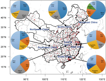
Figure 2. Air quality station incidence and primary crop production levels in major Chinese regions.
Download figure:
Standard image High-resolution imageNormally, high concentrations of ozone precursors accompanied by stable tropospheric air, high temperature, low humidity, and intense radiation are likely to generate severe surface ozone pollution. However, the photochemical reaction process is complicated. For example, the urban NOx emissions react with ozone to generate NO2. Moreover, ozone precursors emitted from urban areas are transported to rural areas through wind and often concentrations are large in rural areas. Wang et al (2007) has found evidence to show that surface ozone concentrations in Chinese rural areas are higher than those in urban areas. Therefore, we probably underestimate rural ozone concentrations since most of air quality monitoring stations are in urban areas.
3. Results
3.1. Surface ozone damages
To select the appropriate functional form for the summary functions (1), we use the shape suggested by an examination of figure 3. That figure shows that marginal damages increase at an increasing rate as surface ozone concentrations increase. Thus, the form  8 was used. The resultant narrow 95% confidence interval and the high levels of R2 (around 0.99) indicate that summary functions effectively represent the CASM marginal damages.

Figure 3. Representative ozone marginal damage summary functions.
Download figure:
Standard image High-resolution image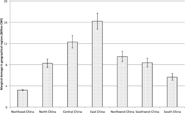
Figure 4. Estimate agricultural damages caused by 2014 ozone concentrations in major Chinese regions.
Download figure:
Standard image High-resolution image
Figure 4 illustrates spatial differences in the damage estimates from the summary functions. Significant disparities arose across seven major regions. For example, marginal damage in East China is more than four times greater than the damages in Northeast China. The economic value of ozone reductions are largest where exposures are high and the region has significant crop production (Westenbarger and Frisvold 1995). The regional differences arise due to crop mix, land area farmed, and ozone levels (see figure 2). Agricultural areas in East China exhibit high ozone concentrations while also growing sensitive crops like wheat and vegetables, for example contributing over 38% of domestic wheat supply. On the other hand, Northeast China that only contributes 0.39% of domestic wheat supply faces relatively smaller impact. In Northeast China and South China, the ozone concentrations are lower plus rice and maize (a less ozone-sensitive crop) account for more than 40% of the planted areas in both regions. These heterogeneous damages suggest spatially differentiated ozone pollution control policies might be attractive although lateral transport of ozone between regions should be considered.
Table 2. National estimates of agricultural damages caused by 2014 ozone concentrations.
| Gross damage | 95% confidence interval | |||||
|---|---|---|---|---|---|---|
| Scenario | Estimate (Billion Yuan) | Fraction of base | Lower bounda (Billion Yuan) | Fraction of base | Upper bound (Billion Yuan) | Fraction of base |
| Subregional marginal damage | 1934.05 | 0.82 | 1629.77 | 0.69 | 2238.32 | 0.94 |
| Provincial marginal damage | 1558.98 | 0.66 | 1419.71 | 0.60 | 1698.25 | 0.72 |
| Linear marginal damage | 2165.06 | 0.91 | – | – | – | – |
aThe lower bound and upper bound of the gross damage is computed based on the 95% confidence intervals of the coefficients in quadratic form of equation (1).
Table 2 presents monetary ozone damage estimates. Total country wide agricultural damages of 2014 ozone concentrations are estimated at CNY 1.9 trillion, or approximately 0.8% of total sectoral associated welfare, and 19% of total agricultural revenue. Table 2 also shows the 95% confidence interval for welfare indicating total damages fall between CNY 1.6 and 2.2 trillion, a welfare loss of no more than 1%.
Table 2 row 2 reports an alternative national damage estimate formed by adding up provincial marginal damages. Notably, this value (CNY 1.559 trillion) is smaller than the summary function results estimated directly over the data set. The difference could be explained by the fact region are weighted equally in adding up the national summary function but not in the estimation. Additionally there are more minimally affected sub-regions than those greatly affected. Thus, simple average damage estimates are somewhat lower.
The third row of table 2 presents aggregate damages constructed following procedures in Muller and Mendelsohn (2007). Namely we multiply the marginal damage at a concentration level in 2014 by the estimated total tons of annual ozone emissions, divided by 2 yielding an estimate of the area below a linear marginal damage line. Figure 3 has shown the concavity of marginal damage curves. Therefore, Muller and Mendelsohn's (2007) method is likely to overestimate the aggregate damages. Thus, the total damage on the basis of linear assumption is CNY 2.2 trillion, which is approximately 24% more than the measures based on the quadratic summary function. This finding confirms that marginal damages are increasing at an increasing rate along the range of surface ozone exposures from figure 3.
We compute the change in total damages of a change in concentrations by subtracting the welfare under the exposure of ozone pollution in 2014 from the one with an alternative level of ozone exposure. By using this direct gross damage measurement, the actual total damage is CNY 1.9 trillion, indicating that our marginal-damage method has minor 1.8% difference. The gap can be attributed to the summary function approach. However, this method is a significant improvement over the piecewise linear marginal damage assumption suggested by Muller and Mendelsohn (2007), which has a measurement error about 14%.
Table 3. Comparisons of output loss estimates caused by ozone exposure by crop, source and year.
| (1) | (2) | (3) | (4) | |
|---|---|---|---|---|
| Aunan et al (2000) 1990 (2020) | Tang et al (2013) 2000 (2020) | Wang and Mauzerall (2014) 1990 (2020) | CASM 2014 | |
| Wheat | 0.0–9.1 (2.9–29.3) | 6.4–14.9 (14.8–23) | 0.8–13 (2–63) | 64.5 |
| Rice | 1.1–1.5 (3.7–4.5) | – | 3–5 (8–10) | 2.3 |
| Maize | 0.0–2.8 (7.2) | – | 1–9.2 (16–64) | 8.9 |
| Soybean | 1.9–11.7 (17.8–20.9) | – | 15–23 (33–45) | 61.2 |
Note: Ecological studies (1), (2), and (3) assume crop planting areas fixed.
Table 4. Country wide estimated benefits of ozone concentration reductions.
| Total | Producers | Consumers | |||||
|---|---|---|---|---|---|---|---|
| Ozone reduction | Total welfare change (Billion CNY) | Fraction of base | Increase rates (%) | Producers' surplus change (Billion CNY) | Fraction of base | Consumers' surplus change (Billion CNY) | Fraction of base |
| –15% | 358.71 | 0.15 | – | −59.41 | −0.05 | 418.12 | 0.33 |
| −30% | 678.21 | 0.29 | 89.07a | −112.83 | −0.10 | 791.04 | 0.63 |
| −45% | 961.47 | 0.41 | 168.03 | −136.15 | −0.12 | 1097.62 | 0.87 |
aIncrease rates are computed through dividing the amount of benefit increments from the first 15% ozone reduction by the gain at the first 15% ozone reduction.
We also compare our damage estimates with results from other relevant studies. Since those studies are agronomic in nature, we only compare crop output losses. Table 3 summarizes the comparison and shows a large difference among the studies. The gap can be attributed to the differing assumptions on ozone concentration and dose response functions (Feng et al 2015). Our results show that our 2014 wheat and soybean losses have reached the levels estimated for 2020 by Wang and Mauzerall (2004). There are two reasons for the larger output losses in our estimates. First, surface ozone exposures in 2014 are much greater than the levels assumed in previous studies. With the rapid industrialization of China, the average daily growing season AOT40 has increased from 558 ppb in 2013 to 621 ppb in 20159, a level which is almost six times the standard defined in the European Union Ambient Air Quality Directive (EEA 2017). Comparing with the assumed AOT40 (15 ppm10) that would occur by 2020 in the Tang et al (2013), East China ozone exposure measured over 90 days (May–July) in 2014 was 62% more than the Tang et al (2013)'s assumption. In addition, CASM optimally alters crop mix which alters output losses. When land is shifted out of wheat and soybean, this raises total output decreases relative to other studies.
3.2. Benefits of surface ozone control
Now we turn attention to the value of ozone concentration reductions. Table 4 shows CASM estimated benefits of systematic reductions from baseline 2014 surface ozone levels. Here we find an ozone reduction of 15% eliminates 19% of the damages while a 30% reduction lowers damages by 35% and a 45% reduction eliminates 50%. This shows diminishing marginal benefits to ozone control and is a result consistent with the findings in Adams et al (1982).
We also examined the income distribution implications of ozone control. Here we found consumers benefit from ozone control but producers are damaged which is a finding contrary to the results in Adams et al (1982) and Adams et al (1989). However we note this is a common finding in the literature (e.g. see Adams et al (1990) and Reilly et al (2003)). Given an inelastic demand curve (which is common in agriculture), prices for farm production will fall when reduced ozone concentrations increase production, and the revenue losses from lower prices often offset productivity gains. In addition, because lower-income consumers tend to spend a larger income share on food they are likely to be the major beneficiaries of surface ozone control.
We also find that not all provinces benefit from ozone control (table 5). Most regions gain from ozone reductions from 2014 baseline ozone levels. However in Guangxi and Hainan under a 30% reduction the producers' loss exceeds the consumers' gain. This is likely due to local soil quality and weather conditions, plus the fact that rice is the dominant crop in these two regions and the consumer group is generally smaller11. Given a surface ozone reduction, the substitution between rice and other profitable crops is limited causing losses of farmers in these two regions to exceed the gains of their relatively smaller number of local consumers. Clearly there will be differential regional effects of ozone control policy.
Table 5. Estimated provincial welfare effects under alternative ozone concentration reduction assumptions.
| Ozone concentration reduction assumption | ||||||
|---|---|---|---|---|---|---|
| 15% Reduction | 30% Reduction | 45% Reduction | ||||
| Province | Surplus (Billion CNY) | Fraction of base | Surplus (Billion CNY) | Fraction of base | Surplus (Billion CNY) | Fraction of base |
| Anhui | 10.66 | 0.10 | 20.48 | 0.19 | 29.60 | 0.27 |
| Beijing | 7.71 | 0.21 | 14.77 | 0.39 | 20.27 | 0.53 |
| Chongqing | 2.18 | 0.04 | 4.55 | 0.08 | 7.12 | 0.13 |
| Fujian | 6.93 | 0.10 | 13.77 | 0.20 | 19.61 | 0.29 |
| Gansu | 3.83 | 0.08 | 7.58 | 0.16 | 12.36 | 0.26 |
| Guangdong | 22.56 | 0.12 | 44.96 | 0.23 | 63.63 | 0.33 |
| Guangxi | −3.24 | −0.04 | −5.12 | −0.06 | −5.95 | −0.07 |
| Guizhou | 2.17 | 0.04 | 4.89 | 0.08 | 8.65 | 0.14 |
| Hainan | −2.34 | −0.15 | −3.71 | −0.23 | −4.31 | −0.26 |
| Hebei | 37.29 | 0.29 | 69.28 | 0.52 | 94.58 | 0.71 |
| Heilongjiang | 4.55 | 0.07 | 9.83 | 0.14 | 14.50 | 0.21 |
| Henan | 31.20 | 0.19 | 57.53 | 0.34 | 79.80 | 0.47 |
| Hubei | 10.31 | 0.10 | 19.79 | 0.19 | 28.55 | 0.27 |
| Hunan | 10.49 | 0.09 | 21.13 | 0.17 | 30.24 | 0.25 |
| Jiangsu | 27.01 | 0.19 | 51.27 | 0.36 | 70.88 | 0.50 |
| Jiangxi | 10.42 | 0.13 | 20.72 | 0.25 | 29.24 | 0.36 |
| Jilin | 8.75 | 0.18 | 17.20 | 0.35 | 24.38 | 0.49 |
| Liaoning | 15.95 | 0.21 | 30.69 | 0.39 | 42.52 | 0.54 |
| Neimenggu | 9.47 | 0.21 | 17.92 | 0.39 | 25.93 | 0.56 |
| Ningxia | 1.16 | 0.10 | 2.16 | 0.18 | 3.21 | 0.27 |
| Qinghai | 0.72 | 0.07 | 1.45 | 0.14 | 2.24 | 0.21 |
| Shaanxi | 4.41 | 0.07 | 6.21 | 0.09 | 9.14 | 0.13 |
| Shandong | 57.47 | 0.34 | 111.26 | 0.63 | 156.76 | 0.89 |
| Shanghai | 7.11 | 0.17 | 13.70 | 0.32 | 18.89 | 0.44 |
| Shanxi | 11.35 | 0.18 | 21.45 | 0.33 | 30.06 | 0.46 |
| Sichuan | 11.18 | 0.08 | 22.09 | 0.15 | 32.79 | 0.22 |
| Tianjin | 5.90 | 0.22 | 11.15 | 0.41 | 15.25 | 0.56 |
| Tibet | 0.96 | 0.17 | 1.87 | 0.33 | 2.60 | 0.46 |
| Xinjiang | 19.67 | 0.49 | 37.03 | 0.90 | 52.07 | 1.27 |
| Yunnan | 1.45 | 0.02 | 4.44 | 0.05 | 8.36 | 0.10 |
| Zhejiang | 14.52 | 0.15 | 27.88 | 0.28 | 38.50 | 0.39 |
Table 6. Estimated effects of ozone concentration reductions on national grain production.
| Ozone reduction assumption | Grain supply (Million ton) | Fraction of base | Rice (Million ton) | Fraction of base | Wheat (Million ton) | Fraction of base | Maize (Million ton) | Fraction of base |
|---|---|---|---|---|---|---|---|---|
| −15% | 29.57 | 5.39 | −0.50 | −0.24 | 25.16 | 19.94 | 4.91 | 2.28 |
| −30% | 57.63 | 10.51 | 0.26 | 0.13 | 48.44 | 38.39 | 8.93 | 4.14 |
| −45% | 91.83 | 16.75 | 0.97 | 0.47 | 78.86 | 62.50 | 12.00 | 5.56 |
Table 7. Estimated effects of ozone concentration reductions on provincial grain production.
| Ozone assumption | |||||||
|---|---|---|---|---|---|---|---|
| 15% Reduction | 30% Reduction | 45% Reduction | |||||
| Province | Base (Million ton) | Output (Million ton) | % Change | Output (Million ton) | % Change | Output (Million ton) | % Change |
| Anhui | 32.07 | 1.82 | 5.66 | 3.12 | 9.72 | 4.96 | 15.47 |
| Beijing | 0.62 | 0.06 | 10.17 | 0.14 | 21.99 | 0.22 | 36.01 |
| Chongqing | 7.84 | −0.03 | −0.38 | 0.00 | −0.06 | 0.06 | 0.82 |
| Fujian | 5.11 | 0.11 | 2.10 | 0.20 | 3.88 | 0.29 | 5.60 |
| Gansu | 8.73 | 1.31 | 15.00 | 2.69 | 30.83 | 4.26 | 48.79 |
| Guangdong | 11.52 | −0.21 | −1.84 | −0.33 | −2.86 | −0.43 | −3.71 |
| Guangxi | 14.12 | −0.26 | −1.86 | −0.32 | −2.24 | −0.33 | −2.36 |
| Guizhou | 8.03 | 0.19 | 2.34 | 0.23 | 2.91 | 0.36 | 4.52 |
| Hainan | 1.53 | −0.08 | −5.46 | −0.15 | −10.10 | −0.22 | −14.39 |
| Hebei | 31.72 | 3.32 | 10.47 | 6.31 | 19.89 | 9.67 | 30.48 |
| Heilongjiang | 55.73 | 0.19 | 0.35 | 0.39 | 0.70 | 0.60 | 1.08 |
| Henan | 55.13 | 6.30 | 11.42 | 11.08 | 20.10 | 16.81 | 30.49 |
| Hubei | 24.14 | 0.92 | 3.81 | 1.69 | 6.98 | 2.56 | 10.60 |
| Hunan | 27.93 | 0.12 | 0.44 | 0.06 | 0.23 | 0.05 | 0.17 |
| Jiangsu | 33.31 | 2.60 | 7.81 | 5.89 | 17.69 | 9.97 | 29.93 |
| Jiangxi | 20.08 | −0.13 | −0.63 | 0.03 | 0.14 | 0.19 | 0.97 |
| Jilin | 33.65 | 0.35 | 1.05 | 0.66 | 1.97 | 0.99 | 2.95 |
| Liaoning | 16.47 | 0.11 | 0.64 | 0.27 | 1.63 | 0.45 | 2.70 |
| Neimenggu | 24.52 | 1.37 | 5.57 | 2.41 | 9.82 | 3.72 | 15.15 |
| Ningxia | 3.27 | 0.23 | 6.92 | 0.43 | 13.23 | 0.72 | 21.93 |
| Qinghai | 0.62 | 0.02 | 3.91 | 0.01 | 0.83 | 0.03 | 4.31 |
| Shaanxi | 10.62 | 1.67 | 15.70 | 4.27 | 40.21 | 7.45 | 70.17 |
| Shandong | 42.90 | 4.49 | 10.47 | 9.53 | 22.21 | 15.74 | 36.70 |
| Shanghai | 1.09 | 0.09 | 8.39 | 0.19 | 17.46 | 0.30 | 27.93 |
| Shanxi | 12.40 | 1.47 | 11.84 | 2.54 | 20.51 | 3.73 | 30.12 |
| Sichuan | 27.39 | 0.66 | 2.41 | 0.88 | 3.23 | 1.43 | 5.23 |
| Tianjin | 1.71 | 0.31 | 18.28 | 0.62 | 36.45 | 0.99 | 57.59 |
| Tibet | 0.94 | 0.00 | 0.01 | 0.00 | 0.05 | 0.00 | 0.10 |
| Xinjiang | 13.47 | 1.31 | 9.71 | 2.28 | 16.96 | 3.41 | 25.29 |
| Yunnan | 15.10 | 0.90 | 5.99 | 1.77 | 11.74 | 2.70 | 17.86 |
| Zhejiang | 6.53 | 0.37 | 5.62 | 0.74 | 11.29 | 1.15 | 17.65 |
Table 8. Emission charges levied on surface ozone precursors.
| Ozone precursor emission chargea | ||||
|---|---|---|---|---|
| Lower boundb | Upper bound | |||
| VOC charge standard (CNY kg−1) | NOX charge standard (CNY kg−1) | VOC charge standard (CNY kg−1) | NOX charge standard (CNY kg−1) | |
| 1.26 | 1.26 | 40 | 10 | |
| Aggregate emmission charge (CNY Billion) | 57.58 | 1204.51 | ||
| % of aggregate damage | 3.31 | 69.25 | ||
aNOX emission is collected from industry in 2014, and VOC emission is the aggregate level from industry in 2012 due to data availability. bPer unit VOC and NOX emmison charge standards are from provincial emission rules in 2015.
3.3. Impacts on domestic grain production
Food security is an important concern and thus we investigate food production impacts (table 6). Generally we find a concentration decrease alters production of rice, wheat, and maize. Specifically, a 45% reduction generates an additional 92 million tons of grain or about 17% above 2014 supply. Wheat accounts for more than 86% of the increase, and maize 13%. Rice production decreases slightly under a 15% reduction but increases under larger ones.
Grain output changes are not spatially uniform (table 7). Hebei, Henan, Jiangsu, and Shandong experience the greatest grain supply increments, and the three southern Guangdong, Guangxi, and Hainan exhibit small decreases because the model switches out of rice toward the more ozone sensitive sugarcane and potato under reduced ozone concentrations.
Columns 3, 5, and 7 of table 7 identify the regions with the greatest increase in grain production due to ozone control. These regions currently have fairly high ozone concentration levels with planted area dominated by ozone-sensitive crops, such as wheat. For example, the seasonal daily AOT40 (May–August 2014) in Shaanxi and Tianjin are 619 ppb and 983 ppb, which are two and three times the concentration in Guizhou, respectively. With a moderate level of ozone reduction (30%), Shaanxi and Tianjin are the most affected regions. Some other regions, like Heilongjiang, Hunan, and Jiangxi, experience almost no impact from ozone control because of their relatively low ozone concentrations and/or cropping patterns dominated by crops not greatly impacted by ozone.
3.4. Discussion on surface ozone control policy in China
This study finds substantial agricultural benefits arise from ozone control along with lower food prices that would benefit consumers particularly the poor. The welfare estimates would need to be compared with the control policy costs although we do not attempt that here. But this comparison would not tell the whole story as the estimates omit health and other benefits. China has begun to control ozone by regulating its precursors imposing regionally specific emission fees. Based on recent provincial ozone precursor regulations, VOC emission charges vary from 1.26 CNY kg−1 to 40 CNY kg−1, and NOX fees from 1.26 CNY kg−1 to 10 CNY kg−1. Table 8 presents estimates optimistic and pessimistic estimates of aggregate surface ozone precursor changes if current highest and lowest standards are implemented, respectively. The lower bound on the monetary gain from such actions is approximately CNY 58 billion, which accounts for 3% of gross damage. The upper bound on the gain is around CNY 1205 billion, which is 69% of the gross damage estimate.
Given the evolution of climate change induced by greenhouse gases will affect atmospheric dynamics and the relationship between ozone precursors and actual ozone concentrations in rural areas as discussed in Lobell and Asseng (2017), the ozone control effort may well have to be a dynamic standard rather than a fixed one.
4. Conclusions
This study has assessed the monetary and production impacts of surface level ozone on China's agricultural sector. Findings show ozone has significant negative national impacts suppressing food production particularly for wheat. Our estimates of the range of total damages falls between CNY 1.6 trillion and CNY 2.2 trillion, which accounts for a loss in total economic welfare in the agricultural sector of approximately 1%. Thus ozone control could help in improving country level welfare and food security. We also find provincial level damages vary across the county which in turn suggests that regionally targeted policies may be appropriate. In particular, perhaps regionally specific ozone pollution standards could be used to address the most damaged areas.
We also studied the benefits and their distribution from ozone control. We found an ozone level reduction of 30% results lowers agricultural sector damages by CNY 0.7 trillion or 35% less. Consumers are the main beneficiaries of reductions, while producers lose. Those losses occur because the decreases in product prices more than offset the increase in supply. Regarding food production, wheat in traditional major grain production provinces is strongly increased under ozone control with maize increased somewhat and rice unaffected.
Furthermore, the reader should note that the damage estimates herein are conservative for several reasons. First they only cover marginal damages in the agricultural sector neglecting effects on human health and other sectors. Second, they may well arise from underestimates of ozone exposure in many rural areas in turn resulting in a lower bound. Third, the lack of China based information on crop sensitivity biases estimates of the crop losses and the corresponding damages which some argue leads to underestimates. Finally, the identification of the most damaged areas is limited by using 2014 observations because lateral transport may heavily confound the adverse effects of surface ozone. For example, regional ozone precursor production may have wide spread and differing cross regional effects due to transmission over distances under variable winds.
Acknowledgments
The authors gratefully acknowledge financial support by the National Science Foundation of China (Grant: 71673137), Nanjing Agricultural University (Grants: SKCX2015004, SKTS2017001), the Priority Academic Program Development of Jiangsu Higher Education Institutions (PAPD), the China Center for Food Security Studies at Nanjing Agricultural University, the Jiangsu Rural Development and Land Policy Research Institute, and the Jiangsu Agriculture Modernization Decision Consulting Center.
Footnotes
- 6
Prefecture level city is a level of administrative division in China that covers agricultural regions.
- 7
CASM covers 16 major field crops including rice, wheat, maize, soybean, peanut, rapeseed, cotton, tobacco, sugarcane, sugar beet, potato, fiber crops, vegetable and cucurbits, other grain crops include oat, barley, sorghum, other beans including all dried beans except soybean, and other oil crops include sunflower and sesame.
- 8
Detailed regression results are available upon request.
- 9
Ozone was added into ambient air quality monitoring system in 2013.
- 10
1 ppm = 1000 ppb.
- 11
The number of residents in Hainan and Guangxi accounts for only 4% of the national population in 2016.