

Abstract
Soil temperature (ST) has a key role in Arctic ecosystem functioning and global environmental change. However, soil thermal conditions do not necessarily follow synoptic temperature variations. This is because local biogeophysical processes can lead to a pronounced soil-atmosphere thermal offset (∆T) while altering the coupling (βT) between ST and ambient air temperature (AAT). Here, we aim to uncover the spatiotemporal variation in these parameters and identify their main environmental drivers. By deploying a unique network of 322 temperature loggers and surveying biogeophysical processes across an Arctic landscape, we found that the spatial variation in ∆T during the AAT≤0 period (mean ∆T = 6.0 °C, standard deviation ± 1.2 °C) was directly and indirectly constrained by local topography controlling snow depth. By contrast, during the AAT>0 period, ∆T was controlled by soil characteristics, vegetation and solar radiation (∆T = −0.6 °C ± 1.0 °C). Importantly, ∆T was not constant throughout the seasons reflecting the influence of βT on the rate of local soil warming being stronger after (mean βT = 0.8 ± 0.1) than before (βT = 0.2 ± 0.2) snowmelt. Our results highlight the need for continuous microclimatic and local environmental monitoring, and suggest a potential for large buffering and non-uniform warming of snow-dominated Arctic ecosystems under projected temperature increase.

Original content from this work may be used under the terms of the Creative Commons Attribution 3.0 licence.
Any further distribution of this work must maintain attribution to the author(s) and the title of the work, journal citation and DOI.
1. Introduction
In the Arctic, climate is warming at twice the rate as lower latitudes, and where the increase in synoptic temperature might have a strong effect on near-surface thermal conditions (Post et al 2009, IPCC 2013). Soil temperature (ST) is fundamentally linked to various aspects of ecosystem functioning, plant growth and reproduction (Bowman and Seastedt 2001, Körner 2003), soil biogeochemistry (nutrient enrichment and microbial activity; Starr et al 2008, Saito et al 2009) and frost-related geomorphological processes (French 2007). Alterations in the topsoil thermal regime were shown to directly modify ecosystem dynamics through changes in both resources and disturbances (Pearson et al 2013, le Roux and Luoto 2014, Paradis et al 2016) and feedback on climate itself either through permafrost degradation and methane release (Blok et al 2011) or through plant redistribution and changes in albedo (Pearson et al 2013, Pecl et al 2017). However, near-surface thermal conditions do not necessarily follow synoptic temperature variations (Geiger et al 2009), with consequences for biotic and abiotic responses to climate warming (Lawrence and Swenson 2011, Lenoir et al 2017). While near-surface soil and air temperatures generally respond to temporal fluctuations in ambient air temperature (AAT) (Pollack et al 2005), locally they can substantially differ due to effects of both physiographic and biophysical processes (Körner 2003, Dobrowski 2011, Lenoir et al 2017) with ST being even more buffered than near-surface air temperature, especially under low vapor pressure deficit (Ashcroft and Gollan 2013). Considering the key role of ST in Arctic ecosystems, such differences may have important consequences on climate feedbacks, but up to now our knowledge of spatiotemporal links between soil and AATs have remained limited. Quantifying the magnitude of the difference between soil and ambient air temperatures and most importantly the biogeophysical processes underlying is necessary to improve projections of changes in STs under anthropogenic climate change, and its subsequent impact on biodiversity redistribution in Arctic ecosystems.
Earlier studies have documented extreme fine-scale variation of ST in Arctic-alpine systems (Scherrer and Körner 2010, Aalto et al 2013). Such soil microclimatic mosaic is attributable to local variation in biogeophysical conditions such as topography, surface soil characteristics and vegetation (Wundram et al 2010, Ashcroft and Gollan 2013, Graae et al 2018). Environmental heterogeneity in these systems is chiefly a direct, as well as an indirect, consequence of local topography (i.e. the mesotopographical depression-ridge-top continuum), controlling snow distribution, snow depth and subsequently soil moisture and vegetation (Billings 1973, Bruun et al 2006, le Roux et al 2013a) (figure 1(a)). Similarly, these factors can be expected to drive the instantaneous soil-atmosphere thermal offset (i.e. the difference between ST and AATs ∆T = ST − AAT; figure 2). For example, ST variations under a thick insulating snow pack are greatly reduced (Grundstein et al 2005), whereas dry soils on wind-exposed ridges abruptly respond to changes in AAT throughout the year due to high vapor pressure deficit (Graham et al 2012, Ashcroft and Gollan 2013). Therefore ∆T can provide an indication of the strength of the 'biogeophysical processes' that mediate AAT and create a heterogeneous soil thermal mosaic over the Arctic landscape (Scherrer and Körner 2010, 2011, Lenoir et al 2013).

Figure 1. General variation in ST and moisture conditions along the mesotopographical gradient (estimated on a ten-point scale) (a) from a local depression (1), mid-slope (5) to a ridge top (10). In the sub-panels, mesotopography was contrasted against: (b) snow depth (cm); (c) mean annual ST (ST, °C); (d) soil moisture (% volumetric water content, VWC); (e) mean summer (June–August) ST (°C); (f) maximum vegetation height (cm); and (g) mean winter ST (°C). The boxplots present median, 1st and 3rd quartiles and 95% range of variation of 322 loggers, while the red line depicts the fitted linear function. The amount of variance explained by the fitted function is expressed as adjusted r-squared (r2) values. Statistical significance of the fit is indicated as ⁎⁎⁎ = p ≤ 0.001. Note the logarithmic scales in panels (d) and (f).
Download figure:
Standard image High-resolution image
Figure 2. Derivation of instantaneous and intra-seasonal soil (ST) - air temperature (AAT) offset (∆T) and coupling (βT). For the sake of clarity, only a random sample of 10 seasonal ST/AAT values (the symbols) were plotted here from a logger located in the North Site (grid 2; see figure 3 for details). The light blue and red lines depict the piecewise ordinary least-square (OLS) regression functions for the AAT ≤ 0 °C and AAT > 0 °C periods, respectively. Both OLS and mean values (colored boxes) are based on all seasonal measurements of the logger.
Download figure:
Standard image High-resolution imageIn recent years, there were attempts to integrate this microclimatic variation into coarse-grained macroclimatic grids by using thermal variability within a spatial unit (e.g. 1 km2) as a proxy for the landscape's potential to buffer against climate warming (Scherrer and Körner 2010, 2011, Lenoir et al 2013). Such an approach can provide an indication of climate resilience or potential for microrefugia (Patsiou et al 2014). However, the general idea of fine-grained and short-distance thermal variability exceeding projected temperature change will allow living organisms to persist within the landscape (Graae et al 2018) does not provide understanding of the environmental factors generating this buffering effect. Another key process involved in macroclimate buffering is the thermal coupling between interior (here soil microclimate) and exterior (i.e. macroclimate or synoptic) conditions (Lenoir et al 2017). Similarly to ∆T, soil-atmosphere thermal coupling, which is the slope parameter of the relationship between AAT and ST (βT; figure 2), is likely to be affected by the local biogeophysical conditions. This suggests that parts of the Arctic landscape can be climatically more stable over time (i.e. more decoupled, low βT values) than others, leading to a spatially uneven local response to changes in macroclimatic forcing. An analysis of time series in combination with direct field measurements of topography, soil and vegetation can provide new insights into the current magnitudes of ∆T and βT and thus the buffering potential in Arctic landscapes.
Here, by using data from a unique network of 322 temperature loggers and climate stations we aim to: (1) uncover the spatiotemporal variation of soil-atmosphere offset (∆T) and coupling (βT) parameters within a topographically complex Arctic landscape; (2) identify the main biogeophysical drivers behind ∆T and βT using field-quantified environmental data within a structural equation modelling (SEM) framework; and (3) use measures of βT to explore the current buffering potential of these topographically rich landscapes in respect to projected climate warming.
2. Materials and methods
2.1. Study site and sampling design
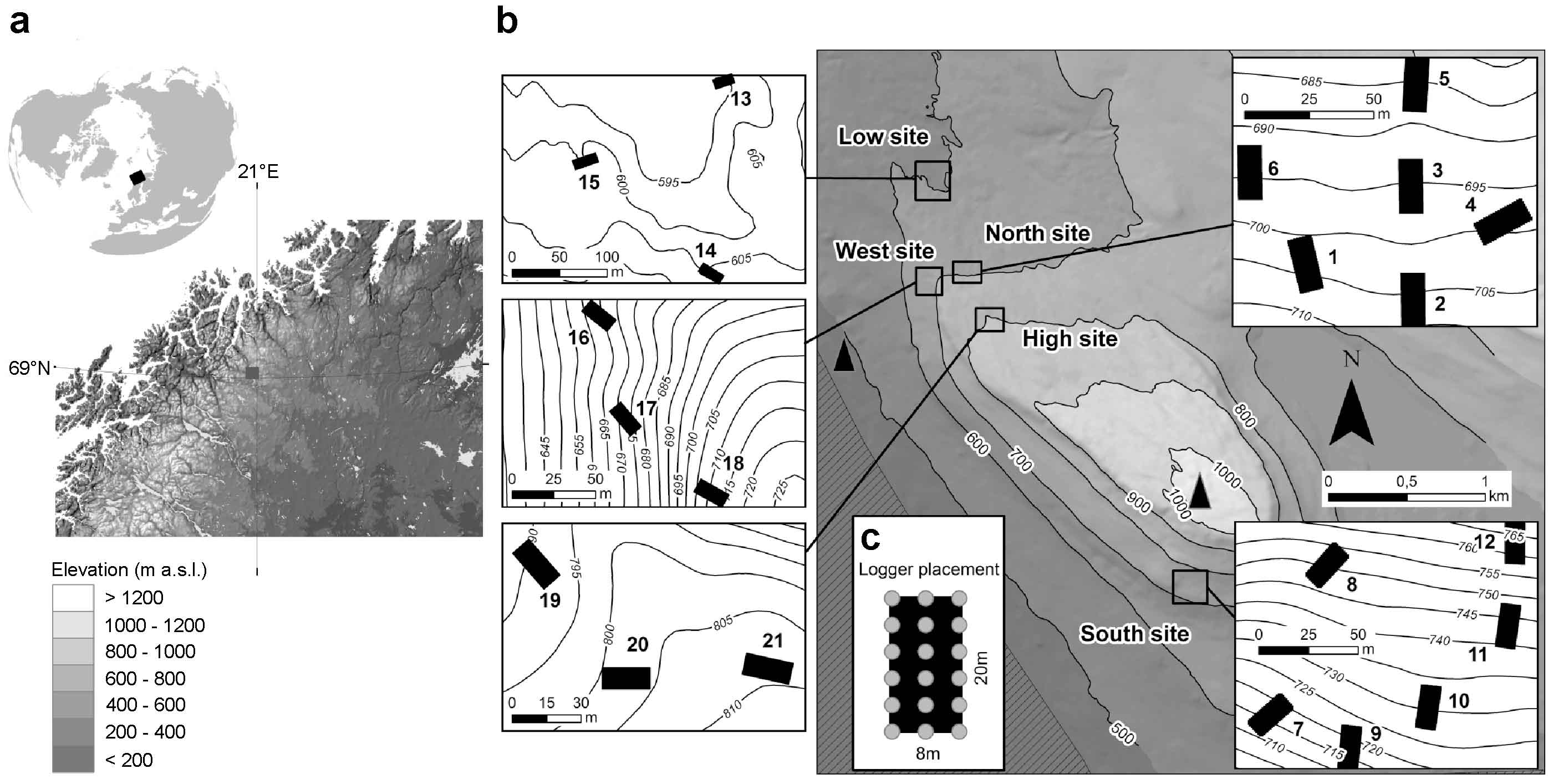
The study was conducted in five sites located within the Saana mountain range in northwestern Finnish Lapland (ca. 69°N, 21°E; figure 3). The sites were located at ca. 600–800 m a.s.l. with different aspects and above the natural treeline (~150 m a.s.l.) formed by mountain birch (Betula pubescens ssp. czerepanovii). Mean annual, January and July air temperatures measured at the nearby Kilpisjärvi meteorological station (69°02'N, 20°47'E, 480 m a.s.l., ca. 1.5 km away) over the period 1981–2010 were −1.9 °C, −12.9 °C and 11.2 °C, respectively. Mean annual precipitation sum was 487 mm over the same period (Pirinen et al 2012). Synoptic temperatures recorded during the study period (2013–2014) were representative of the average conditions during 1981–2010 (figure S1 available at stacks.iop.org/ERL/13/074003/mmedia), while some unusually warm days (i.e. mean daily temperature exceeding the 87.5th percentile of 1981–2010) were observed in August and September 2013. On average, the seasonal snow cover persists until late June (starting from late September) with over 225 days of snow cover. Conditions are favorable for the occurrence of discontinuous/sporadic permafrost (Gisnås et al 2016), although King and Seppälä (1987) showed that the permafrost in this area is likely to be a relict, as shown by the permafrost table being located deeper than 10 m below the soil surface. One can thus reasonably assume that the permafrost is not affecting thermal-hydrological conditions of the topsoil. The study area is topographically complex with surface terrain alternating from local depressions to ridges within distances of tens of meters. The soils consist mainly of glacigenic till deposits, but depending on local topography, bare rocks (summits and steep slopes) and thin organic soils (depressions) are also abundant. The vegetation in the study area is characteristic of Arctic-alpine tundra dominated by shrubs (e.g. Empetrum nigrum ssp. hermaphroditum, Betula nana), graminoids (e.g. Deschampsia flexuosa, Carex bigelowii), mosses (e.g. Dicranum fuscescens) and lichens (e.g. Ochrolechia frigida) with boreal features at lower elevations (le Roux et al 2013b).

Figure 3. Location of the study area in high-latitude Fennoscandia. Panels a and b show the locations of the 21 study grids (8 m × 20 m) across the Saana mountain range, Kilpisjärvi. The positions of the two meteorological stations (MET1, 480 m a.s.l.; MET2, 1009 m a.s.l.) are indicated with black triangles. Panel c shows a schematics of the logger placement (grey circles) at four meter interval in each grid (number of loggers per grid = 18).
Download figure:
Standard image High-resolution imageFor the subsequent analyses, a total of 21 grids (8 m × 20 m, each consisting of 160 adjacent 1 m2 grid cells) were deployed across the five study sites (three on Low, West and High sites, and six on both North and South sites; figure 3). Such a setup was chosen to systematically cover a wide range of environmental conditions, particularly focusing on mesotopography (figure 1(a)). Grids covered 0.34 ha and the distance between the grids varies from ca. 40 m to 3.2 km, with the median distance being 713 m.
2.2. Soil and ambient air temperature data
We recorded annual soil temperature (ST) within each of the 21 grids by using iButton temperature loggers (Thermochron iButton® DS1291G; Dallas Maxim; with a temperature range between −40 °C and 85 °C, resolution of 0.5 °C and accuracy of 1.0 °C). The loggers (originally 378 units) were placed across each study grid at 10 cm below ground and at 4 m intervals (with a total of 18 loggers per study grid; figure 3). Mean horizontal distance between the loggers across the sites varied from 53 m–126 m. Due to technical malfunctions and displacements, only the data from 322 loggers could be retrieved over the studied time period. Loggers recorded STs every four hours from 26 June 2013–25 June 2014.
AAT data (from June 2013–June 2014) were retrieved from two meteorological stations operated by the Finnish Meteorological Institute and located in the vicinity of the study sites (Kilpisjärvi Kyläkeskus meteorological station [MET1], 69°02'N, 20°47'E, 480 m a.s.l. and Saana meteorological station [MET2] 69°2'N, 20°51'E, 1002 m a.s.l.; figure 3).
To characterize the ST regime within the study area, three ST-derived variables were calculated from the time series: annual mean ST (STannual); mean ST over the period with below freezing point AAT (AAT ≤ 0, on average covering 60% of the instantaneous ST measurements); and mean ST over the period with above freezing point AAT (AAT > 0). These two seasons separated by the phase-change point of water intuitively depict a transition from atmospheric conditions favoring snow accumulation and melting. For our definition, these two periods were not limited to consecutive time steps.
2.3. Calculation of the soil-atmosphere thermal offset
The assessment of the soil-atmosphere thermal offset (∆T) included several steps: (1) the instantaneous (i.e. at every time step) AAT lapse rate was determined by calculating the temperature difference between the two meteorological stations (i.e. MET1 and MET2; average difference = −1.8 °C; 90% range of variation = [−9.2; 9.9 °C]); (2) the obtained AAT difference was divided by the 522 m elevation gradient separating the two stations; (3) the AAT for the logger sites were determined based on the instantaneous lapse rate and the average altitude of each grid; and (4) the instantaneous thermal offset (∆Ti = STi − AATi) was calculated for each logger at 4 hour time intervals. Missing values (2% of the annual series) were introduced to the ∆Ti time series due to absent hourly AAT recordings, and were excluded from subsequent analyses. Finally, the ∆Ti were averaged to obtain mean values for two periods (figure 2): AAT ≤ 0 (i.e. ∆TAAT ≤ 0) and AAT > 0 (i.e. ∆TAAT > 0).
2.4. Calculation of the soil-atmosphere thermal coupling
Following Lenoir et al (2017), we measured the soil-atmosphere thermal coupling (βT) by running an ordinary least-square (OLS) regression, where STs of each logger were regressed against AATs (figure 2). However, due to the strong influence of snow depth on STs, we used a piecewise OLS regression approach (Toms and Lesperance 2003) by splitting the annual time series into two distinct seasons: (1) AAT ≤ 0 (i.e. βTAAT ≤ 0); and (2) AAT > 0 (i.e. βTAAT > 0). The resulting slope estimates indicate the agreement between the ST and AAT time series with values close to 1 indicating strong coupling and thus low decoupling.
2.5. Environmental variables
Volumetric soil moisture was measured in all grid cells during the middle of the growing season (16 July 2013) within a time-window of 48 consecutive hours without precipitation using a hand-held time-domain reflectometry sensor (FieldScout TDR 300; Spectrum Technologies, Plainfield, IL, USA) up to a depth of 10 cm, taking the mean of ca. 3 measurements per grid cell (Aalto et al 2013). A recent study by le Roux et al (2013a) indicates that spatial patterns of soil moisture remain relatively constant within and between the growing seasons (Pearson's correlations of repeated measurements > 0.85), thus justifying our use of single measurements in subsequent analyses.
Potential incoming solar radiation (PISR) for both seasons (AAT ≤ 0 [~October–May] and AAT > 0 [~May–October]; MJ cm−2; assuming clear sky conditions) was calculated for each grid cell using the 'Points Solar Radiation' tool in ArcGis 10.3. While the elevation of each grid cell was estimated from a digital elevation model (10 m × 10 m; provided by the National Land Survey of Finland), slope angle and aspect values were measured in the field.
At each grid cell, mesotopography (i.e. a measure of local topography; Billings 1973) was estimated on a 10 point scale (1 = depressions, 5 = mid-slopes, 10 = ridge tops; figure 1(a)). Snow depth (cm) was manually recorded by installing plastic tubes across the study grids at the end of the growing season, which were subsequently measured during the period of maximum snow cover (March 2014). Maximum vegetation height data were collected in July 2011–2013, during the peak of the growing season. Peat depth represents the thickness of the organic layer and was determined by means of three measurements inside each grid cell, using a thin metal rod to probe the soil (Rose and Malanson 2012). Cover of rock represents the percentage of bare rock and coarse gravel within each grid cell.
2.6. Estimation of the landscape's current buffering potential
To explore the potential impact of the current soil-atmosphere βT on STs under warming conditions, we first shifted the seasonal STs according to an AAT warming of +5 °C (i.e. unbuffered ST in equation (1), corresponding to the RCP8.5 emission pathway for the time slice of 2070–2099). Then, βT values were used to multiply the unbuffered ST projections to obtain buffered STs under +5 °C AAT warming (Lenoir et al 2017). Finally, the amount of thermal buffering (k) accounting for decoupling effect between current and future conditions was measured as a relative proportion using the following formula:

where is the arithmetic mean. Thus, a k value close to zero indicates low buffering potential, while a k value close to one suggests a strong buffering potential.

In addition to assess the current buffering potential, we estimated k for AAT ≤ 0 in respect to two alternative scenarios where current snow depths were altered by +50 cm (excluding ridge areas affected by wind transportation) and −50 cm (assuming +5 °C AAT warming). Whereas future increase in water precipitation (and thus less snow accumulation) is commonly expected (Bintanja and Andry 2017), we also examined a possibility for increasing snow depth (i.e. +50 cm scenario), which has been observed in parts of the Arctic (Callaghan et al 2011). We predicted average βTAAT ≤ 0 values at the different snow depth scenarios based on an empirical function (βTAAT ≤ 0 = e−0.99−0.01×snow depth). The current βTAAT ≤ 0 values were adjusted by the average changes in βT when comparing a snow-depth alteration scenario to current conditions. Finally, the k value for a given snow-depth alteration scenario was re-calculated based on the adjusted βT values.
2.7. Statistical analyses
Prior to any statistical analysis, snow depth, rock cover, peat depth, vegetation height and soil moisture variables were log-transformed to approximate normal distributions. The spatial variation in ∆T and βT was related to this list of environmental variables using a structural equation modeling (SEM) framework based on path models (Grace 2006), here as implemented in the R package 'piecewiseSEM', version 1.1.3 Lefcheck (2015). SEM is a statistical modeling technique that combines pathways of multiple predictor and response variables in a single network (Grace 2006). An important difference compared to traditional multiple regression is that, in SEM, variables can appear as both predictors and responses (i.e. endogenous variables), thus allowing for investigation of indirect, mediating or cascading effects (Lefcheck 2015) (figure S2).

Figure 4. Temporal variation in soil and air temperatures, and instantaneous soil-atmosphere thermal offset. Panel (a) shows temporal fluctuation in the annual soil temperature (ST) series with mean (black line), 50%, 95% and absolute ranges (shaded grey-scale polygons). In (b), temporal variation in STs is averaged over three mesotopography levels: depression = 1–2 (mean snow depth = 165 cm); mid-slope = 5 (mean snow depth = 59 cm); and ridge-top = 9–10 (mean snow depth = 19 cm). Panel (c) shows ambient air temperature (AAT) measured at two nearby meteorological stations (MET1 [480 m a.s.l.] and MET2 [1002 m a.s.l.]), and the length of the permanent snow cover measured at MET1 (237 consecutive days with snow ≥ 1 cm, dashed lines). Panel (d) shows temporal variation in instantaneous ST-AAT offset (∆Ti), smoothed using a two-day running mean filter for clarity. The ST data are based on four-hour interval records of temperature for each logger (N = 322) and over a period of one year (from 26 June 2013–25 June 2014). N = number of loggers.
Download figure:
Standard image High-resolution imageDue to the non-independent spatial structure in the data (figure 3), the component models were fitted as linear mixed-effect models (LMMs) using attributes 'Site' and 'Grid' as nested random intercept factors (Bates et al 2014). None of the component models were confounded by multicollinearity as indicated by low variance inflation factor (VIF<2; 'vif' function from the R package 'car', version 2.1–3; Fox and Weisberg 2011). The goodness-of-fit of the SEMs were evaluated using Fisher's C, where p-values for the chi-square > 0.05 indicates a model consistent with the observations (Lefcheck 2015).
The modelling was initiated by defining a full model representing hypothetical causal pathways from the exogenous variables (mesotopography, radiation, and rock cover), through mediators or endogenous variables (snow depth, soil moisture and vegetation) to the response variables (i.e. seasonal ∆T and βT). For ∆TAAT ≤ 0 and βTAAT ≤ 0, the effect of PISRAAT ≤ 0 was not tested due to low direct solar radiations at high latitudes during polar nights that prevails during most of the AAT ≤ 0 period. An error covariance term was defined between peat depth and soil moisture since soil moisture is strongly affected by peat depth. To calibrate each component model, we iteratively (starting from the full model) excluded the most insignificant variable from the models until only significant terms remained (Taka et al 2016). According to Fisher's C statistics, all SEMs provided an adequate fit to the data with C8 = 8.47 (p = 0.39) and C12 = 10.44 (p = 0.58) for ∆TAAT ≤ 0 and ∆TAAT > 0, respectively. For βTAAT ≤ 0 and βTAAT > 0, the corresponding statistics were C8 = 9.24 (p = 0.32) and C6 = 6.98 (p = 0.32), respectively.
3. Results
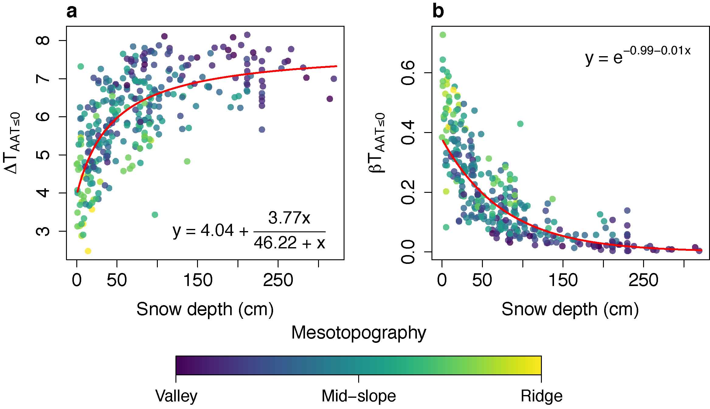
Our data revealed remarkable temporal (figure 4) and spatial (figures 1(b)–(g); tables 1–S1) variations in STs and biogeophysical variables. For example, snow depth was found to vary at most 256 cm and soil moisture 42 % VWC between adjacent logger locations (figure S3(a)). During AAT > 0, STs generally followed AATs, being slightly cooler on average (mean ∆TAAT > 0 = −0.6 °C). However, during AAT ≤ 0, the pattern differed, with STs being, on average, much warmer than AATs (mean ∆TAAT ≤ 0 = 6.0 °C). Similar to absolute STs, notable intra-grid spatial variation in ∆T was observed (figure S3(b); table S2). During AAT > 0, STs were, on average, closely coupled with AATs with βT ranging from 0.50–1.10, while under AAT≤0, βT ranged from 0.01–0.73. The intra-grid spatial variation in βTAAT ≤ 0 and βTAAT > 0 closely followed the relative patterns found for ∆T (table S2). Both ∆TAAT ≤ 0 and βTAAT ≤ 0 showed strong and non-linear relationships with snow depth (figure 5).
Table 1. Summary statistics (N = 322) for soil temperature (ST), soil-atmosphere thermal offset (∆T) and coupling (βT) parameters as well as for several environmental variables. AAT = ambient air temperature, PISR = potential incoming solar radiation, SD = standard deviation, Min = minimum, Max = maximum, VWC = volumetric water content, mesotopo = mesotopography.
| Variable | Unit | Mean | SD | Min | Max |
|---|---|---|---|---|---|
| Soil temperature | |||||
| STannual | °C | 1.8 | 0.7 | −0.4 | 3.4 |
| STAAT ≤ 0 | °C | −1.5 | 1.2 | −5.3 | 0.7 |
| STAAT > 0 | °C | 6.8 | 0.9 | 5.2 | 9.7 |
| Soil-atmosphere thermal offset | |||||
| ∆TAAT ≤ 0 | °C | 6.0 | 1.2 | 2.5 | 8.2 |
| ∆TAAT > 0 | °C | −0.6 | 1.0 | −2.2 | 2.3 |
| Soil-atmosphere thermal coupling | |||||
| βTAAT ≤ 0 | Unitless | 0.20 | 0.15 | 0.00 | 0.73 |
| βTAAT > 0 | Unitless | 0.84 | 0.10 | 0.59 | 1.10 |
| Environmental variables | |||||
| Mesotopo | Index | 5 | 2 | 1 | 10 |
| Rock cover | % m−2 | 12 | 19 | 0 | 94 |
| PISRAAT ≤ 0 | MJ cm−2 | 0.008 | 0.004 | 0.000 | 0.014 |
| PISRAAT > 0 | MJ cm−2 | 0.023 | 0.008 | 0.004 | 0.034 |
| Soil moisture | % VWC | 21 | 11 | 4 | 56 |
| Snow depth | cm | 80 | 69 | 0 | 319 |
| Vegetation height | cm | 17 | 11 | 4 | 80 |
| Peat depth | cm | 5 | 4 | 0 | 24 |

Figure 5. The relationship between snow depth (x-axis) and the soil-atmosphere thermal offset ((a), ∆TAAT ≤ 0 °C) or coupling ((b), βTAAT ≤ 0) parameters (y-axis). The colors represent the loggers' location along mesotopographical gradient from a local depression (purplish colors), mid-slope (greenish colors) to a ridge top (yellowish colors). The red lines depict the fitted non-linear functions. AAT = ambient air temperature.
Download figure:
Standard image High-resolution image
Figure 6. The environmental factors determining the soil-atmosphere thermal offset (∆T) and coupling (βT) processes in the Arctic. For each structural equation model ((a)–(b), for ∆TAAT ≤ 0 and ∆TAAT > 0, respectively; (c)–(d), for βTAAT ≤ 0 and βTAAT > 0, respectively), only statistically significant paths are presented with their standardized path coefficients placed on the arrows. The thickness of the arrows is proportional to the strength of the relationships among variables (red for positive effect, blue for negative effect). The dashed line between the variables peat depth and soil moisture indicates error covariance. The amount of explained variance for component models is reported as conditional R2c based on the variance of both fixed and random terms. AAT = ambient air temperature.
Download figure:
Standard image High-resolution image
Figure 7. The current and projected (under several scenario of changes in temperature and snow depth conditions) thermal buffering potential (k) of an Arctic landscape. The kernel density functions (bandwidth = 0.5) depict the present condition, the unbuffered prediction (+5 °C AAT warming, corresponding to the outcome of emission scenario RCP 8.5 for 2070–2099 across the study area) and the buffered predictions (i.e. predicted future distribution adjusted by soil-atmosphere thermal coupling βT) in soil temperatures (STs) for two seasons: AAT ≤ 0 °C (a) and AAT > 0 °C (b). In addition, for AAT≤0 °C the buffering potential was estimated under two snow-depth alteration scenarios, where observed snow depths were modified by +50 cm and −50 cm, respectively.
Download figure:
Standard image High-resolution image
Path models revealed season-specific networks of factors controlling ∆T (figures 6(a)–(b); figure S4). Mesotopography was found to directly and indirectly control ∆TAAT ≤ 0 through a strong control on snow depth (standardized path coefficient = −0.52) which strengthened the effect of mesotopography on ∆TAAT ≤ 0 (direct effect of snow depth = 0.30, net effect of mesotopography = −0.65). The factors directly influencing ∆TAAT > 0 were more versatile with snow depth (−0.33; indicating the presence of late-lying/perennial snow), soil moisture (−0.28), and vegetation height (−0.12) having a negative effect while rock cover (0.28, partly controlling soil moisture) and potential solar radiation (0.16) having a positive effect. Although no direct effect of mesotopography on ∆TAAT > 0 was found, the net effect was clearly positive (0.21).
During AAT ≤ 0, the network of factors controlling soil-atmosphere thermal coupling (βTAAT ≤ 0) resembled ∆TAAT ≤ 0 with the difference that the direct effect of snow depth was stronger (−0.48) and the direct effect of mesotopography weaker (0.32; figures 6(c)–(d); figure S5). During AAT > 0, rock cover showed the strongest direct effect on βTAAT > 0 (0.36). In addition, βTAAT > 0 was negatively linked to soil moisture (−0.25) and vegetation (−0.16). Although no significant effect of solar radiation was detected, βTAAT > 0 was found to be directly controlled by mesotopography (0.14; in contrast to ∆TAAT > 0).
4. Discussion
Our results provide new insights into the factors determining ST in the Arctic throughout a complex network of biogeophysical processes affecting soil-atmosphere thermal offset (∆T) and coupling (βT). Our study highlights the underestimated thermal variability available across very short spatial distances within Arctic ecosystems, supporting former work on the relevance of small-scale spatial variability in near-surface soil and air temperatures for biotic and abiotic responses under contemporary climate change (Scherrer and Körner 2010, Etzelmüller 2013, Lenoir et al 2013). The data suggest that local topography is a key factor directly (or indirectly throughout the mediating effect of e.g. snow depth) controlling the magnitude of the soil-atmosphere ∆T and βT. Despite the strong influence of snow on ∆T and βT in these systems, multiple other factors contributed to explain ∆T and βT during AAT > 0. For example, the effect of rock cover on ∆T and βT was notable, suggesting rock thermal conductivity to cause a strong coupling of ST with AAT in the topsoil. During warm periods, the excessive heating of rocky surfaces under strong solar radiation can lead to soils being warmer than AAT (i.e. βT >1) with the heat transfer function being reversed (ST warms AAT). In addition, our study confirms the role of soil moisture and vegetation as biogeophysical factors generally smoothing the spatiotemporal variation in STs (through e.g. thermal inertia and reduced net radiation fluxes) leading to notable soil-atmosphere ∆T and βT (Dobrowski 2011, Ashcroft and Gollan 2013).
Our findings suggest that the microclimatic response to meso- and macroclimatic forcing is likely to be altered by biogeophysical processes possibly leading to a non-uniform spatiotemporal soil warming with climate change. We assume that STs under snow cover should, on average, only be slightly affected by changes in AATs, because the very low coupling between soil and air temperatures during that period enhances the buffering potential of the landscape (k = 0.80; figure 7(a)). During AAT > 0, we assume that the average buffering potential should decrease relative to AAT ≤ 0 (k = 0.16) with STs being more coupled with AATs (figure 7(b)).Environmental heterogeneity will cause this buffering potential to substantially vary over the study area (figure S6). Assuming a +5 °C increase in AATs with a βTAAT > 0 ranging from 0.59–1.10, ST warming could vary from +2.5 °C at moist and vegetated depressions to +5.5 °C at dry rocky crests. The outcome of temperature increase in STs being greater, on average, than for AATs would require soils to dry first due to increase in AATs with high vapor pressure deficit in the soil increasing the soil-atmosphere temperature coupling. However, such a situation is unlikely in the Arctic, except at dry rocky crests, due to perennial snow packs acting as soil moisture inputs (Blankinship et al 2014). The buffering potential of STs is especially prominent under AAT ≤ 0 conditions, and in most parts of the landscape, as long as there is snow, the ST response would be highly limited. Accounting for snow distribution is thus of paramount importance to predict the buffering potential of the Arctic landscape according to STs, and thus might contribute to delay the negative impact of macroclimate warming on vegetation and wildlife redistribution (Bertrand et al 2011).
Our analyses only cover the factors controlling intra-annual soil-atmosphere ∆T and βT, which are unlikely to be constant over the years (Lenoir et al 2017). Instead, local environmental conditions related to snow, soil hydrological conditions and vegetation properties are expected to change due to climate warming (Tape et al 2006, Bintanja and Andry 2017). This limits our ability to assess the long-term buffering capacity of Arctic ecosystems, which would require longer time series (≫ three years) of continuous measurements (Lenoir et al 2017). Main uncertainties in the anticipated changes are related to snow and soil moisture dynamics (Räisänen 2008, Pithan and Mauritsen 2014). Recent studies are in consensus that winter conditions (temperature, precipitation amount and phase) are expected to change the most dramatically under future climate change (Callaghan et al 2011, Räisänen and Eklund 2012, Bintanja and Andry 2017). Changes in snow conditions could lead to a highly non-linear feedback where a decrease in snow depth and an increase in days with AAT > 0 (here on average increasing by 88 days assuming +5 °C AAT warming) cause STs to be more strongly coupled with AATs (figure 5). This effect is especially pronounced in parts of the landscape with shallow snow accumulations where βT rapidly responds to small alterations in snow depth (Grundstein et al 2005). Changes in snow and associated ST variation (as seen in figure 4(b)) could thus have effects on physical processes through alterations of wind exposure and soil freezing. Previous studies have also indicated that winter soil thermal conditions have profound carry-over effect on multiple ecosystem properties (soil respiration, nutrient mineralization, carbon cycling and microbial activity) of the following growing season (Wipf et al 2009, Semenchuk et al 2016).
Synoptic temperature data from coarse-grained climatic grids does not capture the near-surface temperature conditions that are relevant for many abiotic and biotic processes (Graae et al 2012, Etzelmüller 2013, Potter et al 2013). Our results of intra-seasonal ∆T indicates that the absolute magnitude of this mismatch was on average >3 °C during our study period, exceeding 8 °C during the AAT≤0 period. The insufficiency of contemporary climate data to describe local STs under future conditions (Williams and Jackson 2007) is further strengthened after considering the effects of βT on soil warming. The cascading effect of ∆T and βT implies that future microclimatic warming trajectories are likely to considerably differ from the ones that are based on coarse-grained climatic grids (Lenoir et al 2017). Here we demonstrate that changes in snow distribution are key to understanding the effects of climate warming in Artic ecosystems. However, it is important to highlight that even during the warm period, remarkable variations in βT within few meters were observed that could contribute to a non-uniform warming across the landscape. Therefore, Arctic ecosystems might be more or less directly affected by changes in atmospheric temperature than expected (e.g. in Post et al 2009, Pearson et al 2013), which may in turn modify current impact projections (in positive or negative ways), suggesting a need for re-assessment of the local rate of climate warming and associated impacts in Arctic regions.
Our findings are highly applicable across snow-dominated Arctic and alpine environments, and highlight the necessity to deploy continuous microclimatic monitoring of both soil and ambient air temperatures, and consideration of fine-scale environmental heterogeneity to support ecosystem impact modelling assessments.
Acknowledgments
J A and M L were funded by the Academy of Finland (project numbers 307761 and 286950). D S and A G obtained support from the Swiss National Science Foundation (grant: 1528661). Authors declare no competing financial interests. Underlying data which support the findings of this study are available from the corresponding author on request.