
Abstract
The fluorescence excitation–emission matrix (EEM) technique coupled with parallel factor (PARAFAC) modeling and measurements of bulk organic carbon and other optical properties were used to characterize the oil components released from the Deepwater Horizon oil spill in the Gulf of Mexico and to examine the chemical evolution and transformation of oil in the water column. Seawater samples were collected from the Gulf of Mexico during October 2010 and October 2011, three months and fifteen months, respectively, after the oil spill was stopped. Together with previous results from samples collected during the oil spill in May/June 2010, these time series samples allow us to elucidate changes in the optical properties of dissolved organic matter (DOM) from the time of maximum oil impact to its recovery, 15 months after the spill. Although the oil had profoundly altered the optical properties of the DOM in the entire water column during the oil spill, naturally occurring DOM became predominant in surface waters by October 2010, three months after the spill. Anomalous DOM with high optical yields, however, still resided in deep waters even 15 months after the oil spill in October 2011, showing a persistent influence of the oil in deep waters. Based on fluorescence EEM data and PARAFAC modeling, three oil components and one natural humic-like DOM could be readily identified. The most prominent oil component had its maximum fluorescence intensity at Ex/Em 224/328 nm, and the other two centered on Ex/Em 264/324 and 232/346 nm, respectively. The humic-like DOM component had its wide emission peak from 390 to 460 nm over the excitation wavelength at ∼248 nm. We hypothesized that component-2 (264/324 nm) was mostly derived from photochemical degradation and the component-3 (232/346 nm) could be a degradation product from both microbial and photochemical degradation, although both C2 and C3 are subject to degradation at different rates. The oil component ratios, such as C2/C1 and C3/C1, were closely related to degradation states of oil and can be used as a sensitive index to track the fate, transport and transformation of oil in the water column.
Export citation and abstract BibTeX RIS

Content from this work may be used under the terms of the Creative Commons Attribution-NonCommercial-ShareAlike 3.0 licence. Any further distribution of this work must maintain attribution to the author(s) and the title of the work, journal citation and DOI.
1. Introduction
The Deepwater Horizon (DWH) oil spill in the Gulf of Mexico from April to July 2010 was an unprecedented marine oil spill event in which over 800 million liters of crude oil gushed from the seafloor at ∼1500 m depth, and a total of ∼7 million liters of dispersants were released into surface and deep waters [1–8]. Massive studies have been carried out to investigate the impacts of oil on ecosystems and factors and processes that regulate the weathering and change of oil composition in the water columns of natural systems [1, 5, 9–11] and in the laboratory [12, 13]. Recent studies have reported the extent and transport of oil, methane and dispersants in the Gulf of Mexico since the DWH oil spill [2, 6, 7, 14, 15]. However, there are no published results on the characterization of oil from seawater samples using fluorescence excitation–emission matrix (EEM) techniques coupled with parallel factor (PARAFAC) analysis. The fate and degradation pathways of oil from the DWH oil spill remain poorly understood. How oil interacts with natural organic matter and the subsequent dynamic changes in chemical and optical properties in the water column after the DWH oil spill in the Gulf of Mexico are largely unknown.
Crude oil contains diverse hydrocarbons and organic molecules that could contribute to UV absorbance and fluorescence signatures in seawater and could be readily determined and characterized by UV–vis spectroscopy and fluorescence spectroscopy techniques [16–21]. Similarly, the composition and sources of dissolved organic matter (DOM) in aquatic environments can be effectively characterized by its optical properties, including UV–vis absorbance and fluorescence EEM spectra [22–30], especially when combining the application of PARAFAC modeling [31–36]. Indeed, fluorescence EEM and PARAFAC techniques have been used in many previous studies to characterize, fingerprint and monitor oil in coastal and marine environments [20, 21, 37–43]. Unfortunately, few studies have been conducted for the DWH oil spill in the northern Gulf of Mexico using the fluorescence EEM technique and PARAFAC modeling to track the fate, transport and transformation of oil in the water column. Our hypothesis was that oil from DWH should significantly alter the optical properties of DOM in the water column and the degradation and transformation processes of oil components could be effectively traced by their dynamic changes in optical properties.
The objective of this study was to examine the dynamic changes in time series bulk organic matter, UV–vis absorbance, and fluorescence EEM spectra in the water column near the Macondo Well in the Gulf of Mexico through cruises from 2010 to 2011 after the oil spill using UV–vis and 3D fluorescence spectroscopy coupled with PARAFAC modeling. Together with data obtained during the oil spill, the variation in oil components and DOM optical properties in the water column over the 15 month time period was used to derive indices for tracking the degradation and transformation processes, and thus the fate and transport of oil in the Gulf of Mexico.
2. Methods
2.1. Study site and sampling
Water samples were collected from stations around the Deepwater Horizon oilrig in the northern Gulf of Mexico during two cruises in October 2010 and October 2011 (figure 1). Both cruises were accomplished onboard the R/V Cape Hatteras and they covered 24 and 27 stations during October 2010 and October 2011, respectively. Detailed sampling locations and selected hydrographic data are listed in table 1.
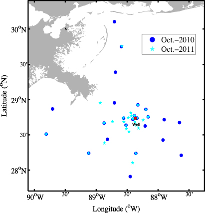
Figure 1. Sampling locations in the northern Gulf of Mexico during October 2010 (blue circles) and October 2011 (teal pentacles) onboard R/V Cape Hatteras. The location of the Macondo Well is shown by a red square.
Download figure:
Standard imageTable 1. Sampling locations, sampling dates, and hydrographic data for stations occupied during October 2010 and October 2011 in the Gulf of Mexico.
| Station ID | Latitude (°N) | Longitude (°W) | Date | Water depth (m) | Surface water temp. (°C) | Surface water salinity |
|---|---|---|---|---|---|---|
| Oct 2010 | ||||||
| GIP 01 | 30°6.113' | 88°42.328' | 10/12/10 | 16 | 24.42 | 31.64 |
| GIP 02 | 29°45.038' | 88°35.618' | 10/12/10 | 28 | 25.46 | 32.92 |
| GIP 03 | 29°23.384' | 88°41.304' | 10/12/10 | 53 | 25.62 | 30.77 |
| GIP 04 | 28°57.278' | 88°56'.103' | 10/14/10 | 126 | 26.30 | 30.26 |
| GIP 05 | 28°52.122' | 89°38'.413' | 10/13/10 | 72 | 26.17 | 30.52 |
| GIP 06 | 28°30.663' | 89°48.499' | 10/13/10 | 530 | 27.11 | 35.36 |
| GIP 07 | 28°14.383' | 89°7.240' | 10/13/10 | 1136 | 27.43 | 35.62 |
| GIP 08 | 27°54.370' | 88°27.001' | 10/14/10 | 2360 | 25.83 | 33.48 |
| GIP 09 | 28°12.581' | 87°37.515' | 10/15/10 | 2530 | 27.27 | 36.41 |
| GIP 10 | 28°25.614' | 87°55.219' | 10/15/10 | 2315 | 26.95 | 36.30 |
| GIP 11 | 28°14.216' | 88°21.528' | 10/16/10 | 1973 | 26.17 | 35.62 |
| GIP 12 | 28°26.275' | 88°49.166' | 10/16/10 | 1210 | 25.96 | 32.70 |
| GIP 13 | 28°40.100' | 88°52.327' | 10/14/10 | 1025 | 26.63 | 32.36 |
| GIP 15 | 28°44.315' | 88°33.390' | 10/16/10 | 1207 | 25.44 | 33.00 |
| GIP 16 | 28°43.383' | 88°24.577' | 10/17/10 | 1560 | 25.66 | 34.26 |
| GIP 17 | 28°38.237' | 88°31.128' | 10/18/10 | 1595 | 25.99 | 34.38 |
| GIP 18 | 28°44.336' | 88°20.416' | 10/17/10 | 1570 | 26.49 | 35.82 |
| GIP 19 | 28°37.587' | 88°12.515' | 10/20/10 | 2010 | 26.99 | 36.43 |
| GIP 20 | 28°45.393' | 88°9.595' | 10/20/10 | 1760 | 26.83 | 36.35 |
| GIP 21 | 28°42.960' | 87°54.086' | 10/20/10 | 2180 | 26.97 | 36.35 |
| GIP 22 | 28°40.502' | 87°39.250' | 10/19/10 | 2370 | 26.97 | 36.28 |
| GIP 23 | 28°51.774' | 88°11.835' | 10/20/10 | 1350 | 25.90 | 34.66 |
| GIP 24 | 28°46.235' | 88°22.874' | 10/18/10 | 1418 | 26.11 | 35.56 |
| GIP 25 | 28°55.602' | 88°19.579' | 10/21/10 | 1160 | 26.05 | 34.99 |
| Oct 2011 | ||||||
| GIP 02 | 29°45.423' | 88°35.125' | 10/20/11 | 20 | 25.28 | 34.58 |
| GIP 04 | 29°45.423' | 88°35.125' | 10/20/11 | 126 | 23.94 | 32.27 |
| GIP 06 | 28°57.252' | 88°56.095' | 10/21/11 | 520 | 26.44 | 36.47 |
| GIP L | 28°30.633' | 89°48.488' | 10/21/11 | 1130 | 26.33 | 35.08 |
| GIP 7 | 28°06.175' | 88°24.657' | 10/21/11 | 1150 | 26.24 | 35.34 |
| GIP K | 28°14.264' | 89°07.380' | 10/21/11 | 1332 | 26.26 | 35.17 |
| GIP 11 | 28°23.047' | 88°52.007' | 10/22/11 | 1984 | 26.20 | 35.39 |
| GIP I | 28°14.255' | 88°21.631' | 10/22/11 | 1734 | 26.19 | 35.51 |
| GIP H | 28°32.779' | 88°28.153' | 10/22/11 | 1697 | 26.21 | 35.47 |
| GIP 17b | 28°35.169' | 88°30.717' | 10/23/11 | 1577 | 26.11 | 35.47 |
| GIP 13 | 28°38.186' | 88°31.018' | 10/23/11 | 1017 | 26.03 | 35.86 |
| GIP M | 28°40.153' | 88°52.284' | 10/23/11 | 1207 | 26.24 | 35.34 |
| GIP G | 28°41.288' | 88°44.181' | 10/23/11 | 1395 | 26.13 | 35.14 |
| GIP 15 | 28°41.113' | 88°33.161' | 10/24/11 | 1178 | 26.12 | 35.35 |
| GIP B | 28°44.331' | 88°33.668' | 10/24/11 | 1480 | 26.11 | 35.32 |
| GIP A | 28°44.593' | 88°28.894' | 10/24/11 | 1237 | 26.22 | 35.40 |
| GIP C | 28°48.874' | 88°26.403' | 10/25/11 | 1378 | 26.03 | 35.42 |
| GIP 24 | 28°46.135' | 88°25.902' | 10/25/11 | 1400 | 25.97 | 35.35 |
| GIP 18 | 28°46.258' | 88°22.852' | 10/25/11 | 1554 | 25.97 | 35.27 |
| GIP 16b | 28°44.304' | 88°20.326' | 10/25/11 | 1554 | 25.88 | 35.27 |
| GIP D | 28°43.788' | 88°24.619' | 10/26/11 | 1618 | 25.84 | 35.23 |
| GIP E | 28°41.365' | 88°22.549' | 10/26/11 | 1708 | 25.89 | 35.28 |
| GIP J | 28°38.349' | 88°21.051' | 10/26/11 | 1847 | 26.15 | 35.34 |
| GIP 23 | 28°35.657' | 88°18.951' | 10/27/11 | 1345 | 25.98 | 35.45 |
| GIP 20 | 28°51.770' | 88°11.777' | 10/27/11 | 1752 | 25.99 | 35.41 |
| GIP F | 28°45.374' | 88°09.595' | 10/28/11 | 1729 | 26.24 | 35.62 |
| GIP 25 | 28°42.65' | 88°14.45' | 10/28/11 | 1150 | 26.09 | 35.46 |
Water samples from different depths at each station were collected with Niskin or Go-flo bottles mounted on a CTD rosette system, including surface waters at ∼2–5 m depth, deepwater samples between 1100 and 1400 m, and bottom water samples (table 1). Immediately after sample collection, the water samples were filtered through pre-combusted glass fiber filters (0.7 μm, Whatman). Filtered water samples for dissolved organic carbon (DOC) were collected in 30 ml HDPE bottles and stored frozen, while samples for optical measurements, including UV–vis absorbance and fluorescence EEMs, were collected with pre-combusted (550 °C) 125 ml amber bottles and stored in the dark at 4 °C.
2.2. Measurements of DOC and UV–vis absorption
Concentrations of DOC were measured on a Shimadzu TOC-V total organic carbon analyzer using the high temperature combustion method [44]. For DOC measurements, samples were acidified with concentrated HCl to pH < 2 before analysis. Three to five replicate measurements, each using 150 μl samples were made, with a coefficient of variance of <2%. Calibration curves were generated before sample analysis. Nanopure water, working standards and certified DOC standards (University of Miami) were measured as samples every eight seawater samples to check the performance of the instrument. Total DOC blank, including water and instrument blanks, was normally less than 2–6 μM [44].
UV–visible absorption spectra of the samples were measured using an Agilent 8453 spectrophotometer and a 1 cm path-length quartz cuvette over the 200–1100 nm wavelength ranges with 0.1 nm increments. The water blank was subtracted, and the refractive index effect was corrected by subtracting the averaged absorbance between 650 and 800 nm [45]. Specific UV absorbance at 254 nm (SUV A254) values were calculated by dividing the absorption coefficient (m−1) at 254 nm (a254) by the DOC concentration (mg C l−1). The non-linear spectral slopes between 290 and 400 nm were calculated to provide information on the overall molecular weight of DOM [30, 46, 47].
2.3. Measurements of fluorescence EEMs
A Shimadzu RF-5301PC spectrofluorometer was used to measure fluorescence signatures of water samples in a 1 cm path-length quartz cuvette. Each sample was scanned from 240 to 680 nm with 1 nm interval under excitation wavelengths from 220 to 400 nm with a 2 nm step. Ninety-one separate fluorescence emission spectra were concatenated to generate an excitation–emission matrix that was able to provide DOM component information for the water sample qualitatively and quantitatively [48, 49]. PARAFAC modeling was used to derive DOM fluorescence components [33] and to examine the spatial and temporal changes in DOM components in the Gulf of Mexico.
A water blank was scanned daily before sample analysis and its EEM was subtracted from each sample's EEM. An emission correction spectrum was generated using Rhodamine B and barium sulfate with the correction package from Shimadzu and multiplied to the EEM spectra. Quinine sulfate standards were also scanned daily for fluorescence calibration and for checking the instrument performance. All fluorescence intensities were converted to ppb-QSE units [49]. Data in two triangular areas, corresponding to the Rayleigh and Raman scattering peaks, were eliminated in the PARAFAC analysis to acquire better mathematical results.
2.4. PARAFAC modeling
PARAFAC modeling was applied to all field seawater samples collected from 2010 to 2011, using MATLAB (MathWorks R2010b) and the DOMFluor Toolbox [33]. Sample matrices were calibrated and corrected before running the PARAFAC analysis. A non-negativity outlier test was performed and no outlier samples were chosen for removal. Thus, no samples were removed before split-half analysis and model validation. The fluorescence intensities of each component in every sample were quantified as a result of the PARAFAC modeling.
3. Results and discussion
3.1. Variations in quantity and quality of DOM in the water column
The spatial distributions of salinity, DOC concentration, UV absorption coefficient at 254 nm (a254) and specific UV absorbance at 254 nm (SUV A254) during October 2010 are shown in figure 2. During October 2010, three months after the oil spill was capped, the DOC concentration and a254 in surface waters did not show an obvious influence of oil and their abundance had dropped back to more naturally occurring levels, with the highest values found at stations close to the Mississippi River plume and a general decrease in DOC with increasing salinity (figure 3).

Figure 2. Distributions of salinity (upper left panel), DOC concentration (mg C l−1, upper right panel), UV absorption coefficient at 254 nm (a254 in m−1, lower left panel) and specific UV absorbance (SUV A254 in m2 g−1 C−1, lower right panel) in the surface water from the northern Gulf of Mexico during October 2010, three months after the oil spill. Note that the Macondo Well is marked with a red square.
Download figure:
Standard image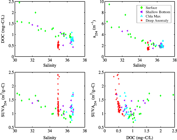
Figure 3. Relationships between salinity, DOC concentration, a254, and SUV A254 in the water column of the northern Gulf of Mexico during October 2010.
Download figure:
Standard imageThese surface distribution patterns are distinctly different from those observed during the oil spill in the May and June cruises [14, 50], showing remarkable resilience of the surface waters. The distributions of DOC and chromophoric dissolved organic matter (CDOM) in surface waters during the early stages of the oil spill in May and June 2010 showed a profound influence of oil released from the Macondo Well in the northern Gulf of Mexico [50], with DOC concentrations as high as 6 mg C l−1 found around the oilrig, which were considerably higher than the baseline values in the northern Gulf of Mexico [44, 51, 52]. Similarly, elevated DOC concentrations and absorbance values in deep waters between 1100 and 1400 m were also observed during May/June 2010 [50], consistent with the presence of oil plume observed in the deepwater [1, 2, 8].
Even though the surface water DOC and CDOM did not seem to have a significant oil signature by October 2010, as shown in figure 2, the relationship between DOC concentration and salinity in all water samples throughout the water column showed an abnormal deviation from a general conservative DOC–salinity relationship as observed before the oil spill in the Gulf of Mexico and in other oceanic environments [24, 44, 53–55]. Surprisingly, some of the DOC concentrations from those abnormal deepwater samples were significantly lower than those observed previously from deep waters in the Gulf of Mexico and North Atlantic Ocean (figure 3 and [44, 51, 52]). We hypothesized that the extremely low DOC concentrations measured for oil contaminated deep waters were the result of the scavenging or removal of DOC by oil droplets and subsequent sorption of oil on the glass fiber filters during water sample filtration.
Based on the correlations between salinity, DOC, a254, and SUV A254, two major types of DOM could be identified in the water column during October 2010, three months after the oil spill (figure 3). The first type of DOM, residing mostly in the upper water column, had natural DOM characteristics with a positive correlation between DOC concentration and SUV A254 values. The second group of DOM, found exclusively in deep waters with a characteristic salinity of 34.96 ± 0.03, had an anomalously high optical yield and a negative correlation between SUV A254 values and DOC concentrations, showing a strong influence of oil on deep waters in October 2010 (figure 3), although rapid recovery was observed in surface waters.
Similarly to the results observed during October 2010 (figures 2 and 3), surface water samples collected during October 2011 (15 months after the oil spill) had undetectable oil signals (figure 4), but deeper water samples again showed a strong presence of oil contaminated DOM (figure 5). While the oil signatures in surface waters identified from optical properties faded away quickly, the presence of oil in the deepwater column persisted even 15 months after the oil spill in the Gulf of Mexico was capped. Effective microbial and photochemical degradation in surface waters, water stratification in the deeper water column, as well as circulation in the Gulf of Mexico [56] are likely the major factors governing the distribution of oil and DOM and their fate and transport in the water column.

Figure 4. Distributions of salinity (upper left panel), DOC concentration (mg C l−1, upper right panel), UV absorption coefficient at 254 nm (a254 in m−1, lower left panel) and specific UV absorbance at 254 nm (SUV A254 in m2 g−1 C−1, lower right panel) in the surface water in the northern Gulf of Mexico during October 2011, 15 months after the oil spill.
Download figure:
Standard image
Figure 5. Relationships between salinity, DOC concentration, a254, and SUV A254 in the water column of the Gulf of Mexico during October 2011.
Download figure:
Standard image3.2. Fluorescence characteristics of DOM in the water column
Fluorescence EEM spectra of crude oil and a time series of seawater samples taken from the same depth at ∼1050 m in the Gulf of Mexico in May 2010, October 2010 and October 2011 are shown in figure 6. The crude oil had its maximum fluorescence emission at 320–360 nm over excitation of 220–240 nm, centering on Ex/Em 226/340 nm. Another peak in the crude oil EEM was located at an emission wavelength of 322 nm under excitation between 260 and 280 nm, similar to that reported by Bugden et al [21].
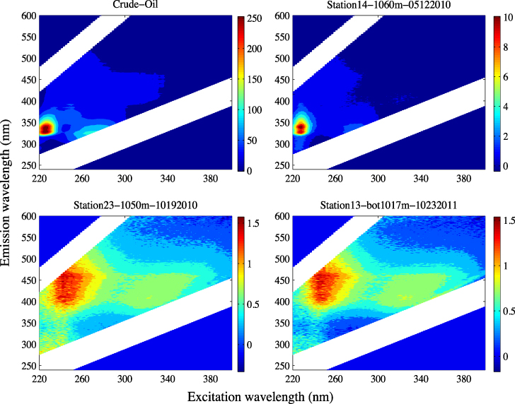
Figure 6. Fluorescence EEMs of crude oil (upper left panel) and seawater samples taken in May 2010 (upper right panel), October 2010 (lower left panel) and October 2011 (lower right panel), respectively. Note that the fluorescence intensity scales are different for the different samples.
Download figure:
Standard imageThe fluorescence EEM signatures of the seawater samples taken in May 2010 strongly resemble those of the crude oil, indicating the presence of oil in the water column and its influence on the seawater samples [50]. However, the oil fluorescence signatures derived from the EEM spectra were weak in the samples collected during the October 2010 and October 2011 cruises (figure 6), indicating effective dilution, degradation and transformation of the oil in the water column. Since the data for DOC and other optical properties clearly demonstrated the presence of oil in deep waters even 15 months after capping the spill (see section 3.1), the weak oil fluorescence signatures observed after the oil spill likely also resulted from the application of a vast quantity of dispersants during the DWH oil spill and thus the interaction of oil with dispersants in the water column [57, 58]. Indeed, significant alterations in oil EEM spectra have been observed when dispersants are present with oil [21, 50, 59]. Other factors contributing to the weak fluorescence signatures included a possible sorption effect during the sample filtration processes since, in general, oil has a very low solubility in seawater, and can be readily removed on filters and sorb on the bottle wall during sample processing.
3.3. Oil components as derived from PARAFAC modeling
Despite low fluorescence oil signatures, oil components could be recognized from these seawater samples using PARAFAC modeling (figure 7). As shown in table 2, four DOM fluorescence components were identified using PARAFAC analysis of EEM data from seawater samples taken during and after the oil spill. A total of 228 fluorescence emission matrices collected at wavelengths from 240 to 680 nm over excitation wavelengths from 220 to 400 nm were decomposed into a four-factor PARAFAC model, including three oil-related components (C1, C2 and C3) and one humic-like DOM component (C4). The first component, C1, having an emission maximum at 224 nm under an excitation wavelength of 328 nm, was the most prominent oil component. The second and third components were identified at Ex/Em maximum wavelengths of 264/324 and 232/346 nm, respectively. The fourth component, with its maximum Ex/Em of 248/446 nm, was characterized as naturally occurring humic-like DOM (table 2, figure 7).

Figure 7. Characteristics of four major DOM components identified by PARAFAC analysis based on fluorescence EEMs of all field samples collected during four cruises from May 2010, during the oil spill (data from Zhou [50]) to October 2011, 15 months after the oil spill in the northern Gulf of Mexico.
Download figure:
Standard imageTable 2. Fluorescent DOM components identified using PARAFAC analysis based on EEM spectra of all field seawater samples collected from the Gulf of Mexico.
| DOM component | Excitation wavelength (nm) | Emission wavelength (nm) | Description |
|---|---|---|---|
| Component-1 | 224 | 328 | Oil |
| Component-2 | 264 | 324 | Oil |
| Component-3 | 232 | 346 | Oil |
| Component-4 | 248 | 446 | Humic-like |
As shown in figure 8, the fluorescence intensities of the oil component C3 had a broad correlation with a254 in the Gulf of Mexico in October 2010, suggesting an oil component with similar quantum yields and optical activities. A more scattered relationship between a254 and the fluorescence intensities was observed for oil components C2 and C1 (figure 8), suggesting that both C1 and C2 were more complex in composition and might have multiple production/degradation pathways.
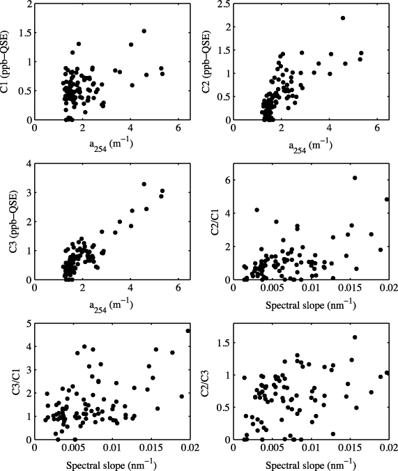
Figure 8. Relationships between a254 and the fluorescence intensities of oil components C1, C2 and C3 and between the spectral slope (S) and oil component ratios C2/C1, C3/C1 and C2/C3 in the water column of the northern Gulf of Mexico during October 2010.
Download figure:
Standard image3.4. The chemical evolution of oil as characterized by its component ratios
Since the oil-related fluorescence components identified by PARAFAC modeling were derived from seawater samples collected at different times during and after the oil spill, changes in the fluorescence intensities and component ratios between seawater samples would likely reflect the results of degradation and transformation of the oil in the water column. Additionally, the fluorescence component ratio is an intensive property, which is not related to the quantity or abundance of oil, and should be an ideal parameter or index to evaluate time series samples in the same water column. As shown in figure 9, even though the intensity/concentration of DOM fluorescence components decreased with time, the C2/C1 and C3/C1 ratios increased consistently in seawater samples from the middle of May to May/June to October 2010 and to October 2011, indicating that these oil component ratios are indeed correlated with oil degradation and can be used as an index for tracking the chemical evolution of the oil during its degradation and transformation in the water column. The increase in the C2/C1 and C3/C1 ratios during oil degradation in the water column suggested that the two oil components C2 and C3 had significantly lower degradation rates as compared to the C1 oil component, or that C2 and C3 were also degraded products of crude oil. Independent controlled laboratory experiments on the degradation of crude oil also provided similar variation trends of oil component ratios with increasing C2/C1 and C3/C1 ratios during oil degradation [50], further supporting the use of C2/C1 and C3/C1 ratios as an index to trace weathered and degraded oil in marine environments.

Figure 9. Variations in the oil component ratios, C2/C1 and C3/C1, with time based on field samples collected during four cruises at different times in the Gulf of Mexico, including samples taken in mid-May 2010 [M10] and late May–early June 2010 [MJ10] during the oil spill (data from [50]), October 2010 [O10] three months after the oil spill, and October 2011 [O11] 15 months after the oil spill was capped. Deepwater samples are denoted with purple squares, while surface water samples are denoted with green pentacles.
Download figure:
Standard imageData from the October 2010 cruise also show a broad correlation between spectral slope values and oil component ratios such as C2/C1, C3/C1 and C2/C3 in the water column of the Gulf of Mexico although the correlations are somewhat scattered (figure 8). Given that the spectral slope values are inversely related with the aromaticity and average molecular weight of DOM [30, 46], these positive correlations between oil components and spectral slope values suggested that C2 and C3 were less aromatic, lower inferred molecular weight components compared with crude oil. Thus, the overall molecular weight of DOM in the water column is expected to decrease as the oil is degraded and as the C2/C1 and C3/C1 ratios increase (figure 9). A similar correlation between the C2/C3 ratio and the spectral slope (figure 8) further suggests a decreasing trend of average molecular weight in oil components from C1 to C3 and then to C2. However, detailed analyses of hydrocarbon composition are needed to confirm this conclusion derived from spectral slope measurements.
Interestingly, the C2/C1 ratios in surface water samples were, in general, slightly higher than those in deepwater samples regardless of sampling time, suggesting that either the C2 component was less sensitive to photochemical degradation, or its production rate from degradation was slightly higher than its degradation. In contrast, surface water C3/C1 ratios were in general lower than deepwater samples except for the May 2010 samples collected during the oil spill (figure 9), suggesting that the production of C3 in the surface waters could be lower than its degradation. We hypothesize that C2 is mostly derived from photochemical degradation and C3 is a degradation product from both microbial and photochemical degradation, while both of them are also subject to degradation in the water column. The inferred C2/C3 ratio was higher in surface water samples than in deep waters, and increased with time, which further confirmed the degradation preference of C2 and C3. Thus, changes in oil component ratios in the water column could be quantitatively linked to the fate, degradation and transformation pathways of crude oil in the water column.
4. Conclusions
The Deepwater Horizon oil spill had a profound influence on the optical characteristics of DOM in the northern Gulf of Mexico. At the early stages of the oil spill, more freshly released crude oil in the water column gave rise to elevated DOC concentration and optical reactivity, showing two distinct types of DOM in the water column, with a strong influence of oil throughout the entire water column. During October 2010, three months after the oil spill was capped, the DOM in the upper water column seemed to contain mostly natural organic matter. However, anomalous DOM with high optical yields still resided in deep waters, showing a persistent oil influence on the optical properties. The strong presence and persistent influence of oil in the water column was also observed in deep waters surrounding the Macondo Well even during October 2011, 15 months after the oil spill had been capped. Four DOM fluorescence components were identified using PARAFAC modeling on EEM data of seawater samples from the Gulf of Mexico. Three of them were oil components and one was UV humic-like DOM. The fluorescence component ratios, such as C2/C1 and C3/C1, showing a consistent increase with increasing time from 2010 to 2011 in the Gulf of Mexico, could be quantitatively linked to the degradation status of the oil in the water column and thus be used as indices to effectively track the fate and transport of oil in marine environments. These results have important implications in oil spill research, environmental monitoring, and the development of in situ sensors.
Acknowledgments
We thank Hailong Huang and chief scientists, captains, crewmembers and scientists onboard R/V Pelican, Walton Smith and Cape Hatteras for their help in sample collection, Dr Huijun He for his assistance in sample analysis using fluorescence spectroscopy, and David Rosenfield for critical reading of the paper. This study was supported in part by grants from NSF-RAPID (OCE#1232491 and #1042907), RAPID-MRI (#1057726), and GoMRI/BP through NGI (project #11-BP_GRI-21 and 11-BP_GRI-22).