
Abstract
Global land use research to date has focused on quantifying uncertainty effects of three major drivers affecting competition for land: the uncertainty in energy and climate policies affecting competition between food and biofuels, the uncertainty of climate impacts on agriculture and forestry, and the uncertainty in the underlying technological progress driving efficiency of food, bioenergy and timber production. The market uncertainty in fossil fuel prices has received relatively less attention in the global land use literature. Petroleum and natural gas prices affect both the competitiveness of biofuels and the cost of nitrogen fertilizers. High prices put significant pressure on global land supply and greenhouse gas emissions from terrestrial systems, while low prices can moderate demands for cropland.
The goal of this letter is to assess and compare the effects of these core uncertainties on the optimal profile for global land use and land-based GHG emissions over the coming century. The model that we develop integrates distinct strands of agronomic, biophysical and economic literature into a single, intertemporally consistent, analytical framework, at global scale. Our analysis accounts for the value of land-based services in the production of food, first- and second-generation biofuels, timber, forest carbon and biodiversity. We find that long-term uncertainty in energy prices dominates the climate impacts and climate policy uncertainties emphasized in prior research on global land use.
Export citation and abstract BibTeX RIS

Content from this work may be used under the terms of the Creative Commons Attribution-NonCommercial-ShareAlike 3.0 licence. Any further distribution of this work must maintain attribution to the author(s) and the title of the work, journal citation and DOI.
1. Introduction
The allocation of the world's land resources over the course of the next century has become a pressing research question. Continuing population increases, improving diets amongst the poorest populations in the world, increasing production of biofuels, and rapid urbanization in developing countries are all competing for land, even as the world demands more land-based environmental services [1, 2]. Land use changes are also an important driver of global greenhouse gas (GHG) emissions. From 1850 to 1998, about 500 GtCO2e were emitted as a result of land use change, predominantly from forest ecosystems, contributing to about one third of total GHG emissions over this period [3]. Managing anthropogenic carbon emissions from terrestrial systems is thus a key avenue for limiting atmospheric carbon dioxide (CO2) concentrations to low levels [4]. However, agriculture and forestry are also vulnerable to climate change, which alters the biophysical environment for land-related activities [5–9]. This combination of intense competition for land, coupled with great uncertainty about future productivities and the valuation of environmental services, gives rise to a significant problem of decision making under uncertainty [10]. Understanding the potential impact of these uncertainties is critical for policy makers to assess the possible consequences of different decisions, including that of inaction [11].
Most research to date has focused on quantifying uncertainty effects of three major drivers affecting competition for global land use. The first of these effects is the uncertainty in energy and climate policies affecting competition between food and biofuels [12–16]. The second is uncertainty about climate change impacts on yields and available area in agriculture and forestry sectors [6–9, 17–22]. The third of these is the uncertainty in technological change affecting the efficiency of food, bioenergy and timber production [2, 23–27]. One source of uncertainty that has received relatively less attention in the literature is the uncertainty in the market price for fossil fuels. Petroleum and natural gas prices are key factors affecting competitiveness of biofuels [28, 29] as well as the price of nitrogen fertilizer which is critical for boosting agricultural yields [30]. Rising energy prices thus put significant pressure on global land supply and greenhouse gas emissions from terrestrial systems.
The goal of this study is to compare the effects of these core uncertainties on the optimal profile for global land use and land-based GHG emissions over the next century. Our analysis is based on a dynamic long-run, forward-looking global partial equilibrium model, in which the societal objective function places value on production of services from food, liquid fuels (including first- and second-generation biofuels), timber, forest carbon and biodiversity. This fully intertemporal treatment of global land use distinguishes the present study from all of those cited above, and brings new insights regarding the path of optimal land use over time. Such an intertemporal treatment is essential if one is to properly characterize the optimal time path of forestry production [31]. And, as we will see, it is also critically important in understanding the dynamic impacts of climate policies.
We find that the effect of uncertainty in energy prices on global land use in 2100 is considerably larger than in the existing analyses of global land use which have largely focused on energy and climate mitigation policies as well as climate impacts. Our model predicts that long-run sensitivity of the optimal path for global crop land for food and biofuels' feed stocks with respect to variation in energy price forecasts is four times higher as compared to variation in predicted climate impact on agricultural yields, and two times higher as compared to variation in GHG emissions targets.
2. Methodology
The analysis used here employs FABLE (Forest, Agriculture, and Biofuels in a Land use model with Environmental services), a dynamic optimization model for the world's land resources over the next century. This model brings together recent strands of agronomic, economic, and biophysical literature into a single, intertemporally consistent, analytical framework, at global scale. The model solves for the dynamic paths of alternative land uses, which together maximize global economic welfare, subject to a constraint on global GHG emissions. A brief description of the model follows, with complete information offered in the model's technical documentation [32].
2.1. Model description
FABLE is a perfect foresight, discrete dynamic, finite horizon partial equilibrium model. It seeks to determine the optimal allocation of scarce land across competing uses and across time. As such, it reflects incentives faced by forward-looking, profit-maximizing investors, as well as their responses to alternative states of the world, including climate change, GHG emissions polices and energy prices.
Figure 1 summarizes the model's structure. There are two natural resources in the model: land and fossil fuels (oil and natural gas). The supply price of fossil fuels follows an exogenous path which is uncertain. The supply of land is fixed and faces competing uses that are determined endogenously by the model. We distinguish between five types of land: unmanaged forests, protected forests, commercial forests, and cropland dedicated to food crops and cellulosic feedstocks. Unmanaged forests are natural lands in an undisturbed state. These lands can be accessed at some cost and thereupon converted to commercial land (deforested) or to protected forest land. Institutionally protected lands include natural parks, biodiversity reserves and other types of protected forests. These lands are best used to produce ecosystem services for society and cannot be converted to commercial lands. Commercial lands are used in either agriculture or forestry. Agricultural lands grow food crops (which can also be converted to first-generation biofuels), and cellulosic feedstocks used exclusively in production of second-generation biofuels. Commercial forests yield timber and GHG abatement benefits and are characterized by multiple tree vintages, which can be harvested for producing timber products or left to grow, contributing to GHG abatement by forest sinks.
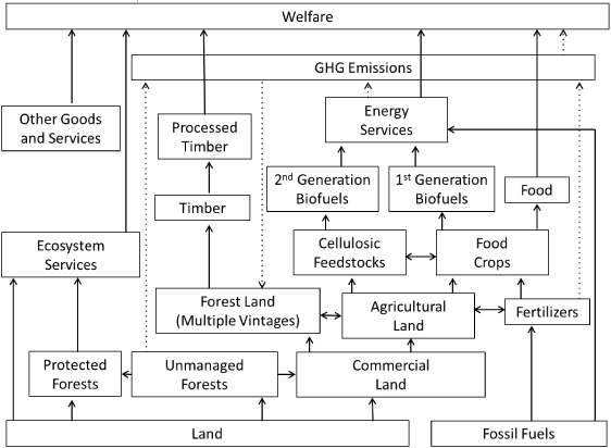
Figure 1. Structure of the FABLE model.
Download figure:
Standard imageWe analyze eight sectors producing intermediate and final goods and services, including: agrochemicals, crop production, food processing, biofuels, energy, forestry, timber processing, and ecosystem services. The agrochemical sector converts fossil fuels into fertilizers that are used to boost yields in the agricultural sector. The farm sector combines cropland and fertilizers to produce agricultural output that can be used to produce food or biofuels. The food-processing sector converts agricultural output into food products that are used to meet global food demand. The biofuels sector converts agricultural products into liquid fuels, which substitute for petroleum products. We consider two types of liquid biofuels: first-generation biofuels (e.g., corn-based ethanol), which substitute imperfectly for petroleum in final demand, and second-generation biofuels (e.g., cellulosic biomass-to-liquid diesel obtained through Fischer–Tropsch gasification), which offer a 'drop-in' fuel alternative3. The energy sector combines petroleum products with first- and second-generation biofuels, and the resulting mix is further combusted to satisfy the demand for energy services. The forestry sector produces an intermediate product, which is further used in timber processing. The timber-processing sector converts output from the forestry sector into a final timber product, which satisfies commercial demands for lumber and other articles of wood. The ecosystem services sector combines different types of land to produce terrestrial ecosystem services4. The production of non-land-based goods and services is predetermined. Other exogenous drivers of global land use include: population growth, global per capita income, oil prices, climate change, and technological progress, which captures yield improvements in agriculture and forestry, and more efficient use of services from food and timber processing, energy, and recreation sectors.
GHG emissions flows in the model result from a number of sources: (a) combustion of petroleum products, (b) the conversion of unmanaged and managed forests to agricultural land (deforestation), (c) non-CO2 emissions from use of fertilizers in agricultural production, and (d) net GHG sequestration through forest sinks (which includes the GHG emissions from harvesting forests). We calculate GHG emissions using exogenous conversion factors corresponding to each of these (endogenous) sources. Further details are available in the model's technical documentation [32].
The societal objective function being maximized places value on processed food, energy services, timber products, and ecosystem services. Emissions of greenhouse gases (GHGs) are central to the problem at hand, and are accordingly treated as a time-varying constraint on the flow of GHG emissions (i.e., 'emissions target').
2.2. Scenarios
We apply our model to analyze the comparative dynamics of global land use under different scenarios to assess the significance of uncertainties in energy prices, climate change impacts on agriculture, and climate policies. Figure 2 summarizes these scenarios. Our baseline scenario reflects projections from a number of international agencies and assumes: population growth will plateau at 10 billion people by 2100 [33], global per capita income will rise at a rate of 2.25% yr−1 [34], oil prices rise at 3% yr−1 over the twenty first century [35], introduction of new energy efficient technologies [36], and finally, GHG/warming at the rate of 0.3 °C/decade [37]. We assume that all of the alternative scenarios are first realized after 20 years from the 2005 starting period, i.e. 2025.
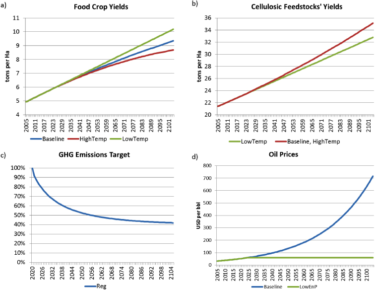
Figure 2. Model scenarios. Panels (a) and (b) pertain to climate change impacts. Panel (c) pertains to GHG regulatory scenario and panel (d) shows energy price scenarios.
Download figure:
Standard imageClimate change scenarios HighTemp and LowTemp affect agricultural yield growth (figure 2(a)) and are based on the range of uncertainty in global temperature increases from IPCC SRES climate scenarios [37]. We consider separately the effects of climate change on food crops, (e.g., grains and oilseeds), and on cellulosic feedstocks for production of second-generation biofuels. These two types of agricultural products differ in important ways. The impact of temperature on food crop yields depends critically on their phenological development, which, in turn, depends on the accumulation of heat units, typically measured as growing degree days (GDDs). More rapid accumulation of GDDs speeds up phenological development, thereby shortening key growth stages, such as the grain filling stage, hence reducing yields [38]. In contrast, with second-generation feed stocks, such as switchgrass, the entire aboveground biomass is harvested for biofuel. Higher temperatures favor overall biomass development. Yields increase strongly under moderate climate change and appear to be relatively insensitive to further temperature increases [39]. These gains are further reinforced with increased CO2 concentrations, which benefit both types of feedstocks by reducing water stress [39].
Scenario HighTemp is designed to capture a worst case scenario. It assumes 0.6 °C temperature increases per decade with no gains from CO2 fertilization, whereas scenario LowTemp assumes just 0.1 °C temperature increase per decade, and accounts for maximum benefits from CO2 fertilization. There is a considerable variation in the biophysical and agronomic literature on the range of climate impacts on global food crop yields. The results of recent biogeochemical, climate, and dynamic crop vegetation model simulations [18, 21, 22], and regression-based methods [6, 8, 20] suggest a range of yield responses in 2100 of about 15–20% under different climate scenarios. In this study we use results from the statistical methods, and estimate that food crop yields would be 8% above baseline in 2100 under scenario LowTemp, whereas scenario HighTemp leads to a 7% decline in yields relative to 2100 baseline (figure 2, panel (a)).
As a robustness check we also obtained results from runs of the Decision Support System for Agrotechnology Transfer (DSSAT) crop simulation models [40], run globally on a 0.5° grid and weighted by agricultural output under maximal (representative concentration pathway 8.5) and minimal (representative concentration pathway 2.6) GHG forcing scenarios using outputs taken from the CMIP5 archive [41] for the HadGEM2-ES [42] and IPSL-CM5A-LR [43] climate models. The results of the crop simulation model suggest an asymmetric distribution of losses ranging from 0 to −25% of historical yields for maize, and more modest losses, with the potential for modest gains in the case of soybeans [44, 45]. Combining these two sets of results, we believe that the 15% variation in aggregate yields food crop shown in figure 2(a) is reasonable.
Because evidence of climate impacts on cellulosic feed stocks is not yet well established, we employ the results of small scale laboratory experiments in Midwestern United States [39]. We assume that cellulosic feedstock yields benefit less from lower temperature growth and more modest CO2 fertilization impacts, resulting in yields that are 50% lower than baseline under scenario LowTemp, while remaining unchanged in scenario HighTemp (figure 2, panel (b)).
The GHG regulation scenario (Reg) is illustrative of the range of regulatory uncertainty surrounding global GHG emissions based on IPCC 4AR projections [46, 47]. In this scenario we introduce a maximum target dictating a 60% reduction in baseline GHG emissions from petroleum products, crop production and terrestrial carbon fluxes by 2100. This corresponds to the upper bound of regulation, aimed at achieving CO2 equivalent concentration (including GHGs and aerosols) at stabilization between 445 and 490 ppm. After the target is introduced, it rapidly becomes more stringent, with larger GHG emissions' reductions taking place by 2050 (figure 2, panel (c)). The baseline scenario assumes no regulatory policies, and thereby reflects a lower bound with respect to this instrument.
In order to characterize the extent of energy price uncertainty, we begin with the US Energy Information Administration (EIA) growth projections for 2035 [35], which range from $62/bbl to $200/bbl, with an expected value of $145/bbl. The latter implies an annual growth rate of 3% per year as of model reference year 2004. In our baseline scenario, oil prices continue to grow at this rate throughout the century, reaching $700/bbl by 2100. In our low price scenario, LowEnP, these prices remain flat throughout the period (figure 2, panel (d)). This large range of change in energy prices reflects uncertainties in extraction costs, demand for fossil fuels, government policies of petroleum producing countries, and discovery and development of new oil fields. As a robustness check, we will also explore lesser ranges of energy price uncertainty, thereby permitting us to ask what more limited oil price ranges imply for global land use.
3. Results
3.1. Model baseline
Figure 3 shows the optimal paths of global land use (panel (a)) and GHG emissions (panel (b)) over this century in the baseline scenario, which is characterized by steady growth in energy prices and agricultural yields, and the absence of climate policies. Land area dedicated to food crops expands, reaches its maximum of 1.85 GHa in 2040 due to increasing population and evolving consumption patterns. It declines thereafter as population and per capita demand growth slow, and are overtaken by technological progress in agriculture. Protected forests expand rapidly in the second part of this century in response to growing consumer demand for ecosystem services as households become wealthier. Compared to 2005 levels commercial forest area expands by 10%, reaching 1.8 GHa in 2100 to satisfy the growing demand for wood products, worldwide, while unmanaged forest areas give way to protected and commercial forests and shrink by 25%, accounting for 1.85 GHa in 2100. With steadily rising oil prices, land devoted to biofuels expands gradually—particularly after second-generation biofuels become commercially competitive in 2040, with feedstocks occupying 210 MHa in 2100.

Figure 3. Optimal paths of (a) global land use and (b) GHG emissions in model baseline.
Download figure:
Standard imageFigure 3(b) shows annual GHG emissions flows from land use and related sectors. Positive bars in this panel denote emissions, whereas negative bars denote carbon sequestration through forests and petroleum emissions displaced by less carbon-intensive biofuels. GHG emissions from land use and related sectors decline considerably in the long-run, even in the absence of binding climate policies. This is simply a function of baseline technological progress, which enables more food, energy and forest services to be obtained from the same amount of land. GHG emissions from production and application of fertilizers also decline steadily, as their production costs increase and pressure on croplands diminishes in the face of slowing global population growth and improving crop technology. GHG emissions from conversion of natural land remain significant in the short-run, and the medium-run.
In the long term, increasing access costs of natural land combined with declining demand for commercial land, results in a sharp decline in deforestation. Annual GHG emissions from deforestation decrease to 1.3 GtCO2e yr−1 in 2050 (67% smaller compared to 2005) and cease entirely by 2065, along this optimal global path of land use. GHG emissions' sequestration does not change significantly in the short- and medium-run under the no-climate policy scenario. In the long-run, establishment of more extensive area in commercial forest offers a one-time increase in sequestered GHG emissions. In 2100, annual GHG abatement owing to forestry amounts to 4.35 GtCO2e yr−1, which is about 1.5 times larger than 2005. Rapid expansion of second-generation biofuels contributes to a reduction in global GHG emissions due to the 75% offset (based on GREET fuel-cycle model fleet calculator [48]) when compared to petroleum combustion. Annual GHG emissions savings from biofuels' offsets (ignoring indirect land use effects, which are recorded separately) amount to 1.55 GtCO2e yr−1 in 2100. This is much smaller than projections from land-based integrated assessment models [13, 15, 23, 49]. Our analysis however is limited to liquid biofuels, and ignores other end uses of bioenergy, such as heat and electricity generation, which have a significant potential for land-based climate abatement [23].
3.2. Land use change sensitivities
Figure 4 reports the simulated range of land use changes for food crops and biofuels' feedstocks relative to the model baseline for the climate impact scenarios, LowTemp and HighTemp, GHG regulation scenario, Reg, and energy prices, LowEnP. Higher temperatures lead to a decline in agricultural yields for food crops and result in greater requirements for cropland and fertilizers to produce food and first-generation biofuels. In 2100, the cropland area increases further by 37 MHa, or about 2.5%, in the HighTemp climate scenario, relative to baseline. This increases the competition for land with second-generation biofuels, which is diminished by an additional 10 MHa, or 5% under scenario HighTemp. Lower temperatures result in lower yields of cellulosic feed stock, and therefore greater requirements for land and fertilizers used in producing second-generation biofuels. Compared to the baseline scenario, the land area dedicated to biofuels increases by 19 MHa, or by 9% in scenario LowTemp by 2100. Overall, uncertainty in climate impacts results in a variation of land use change for food crops and biofuels' feed stocks in 2100 of about 100 MHa (figure 4(a)).
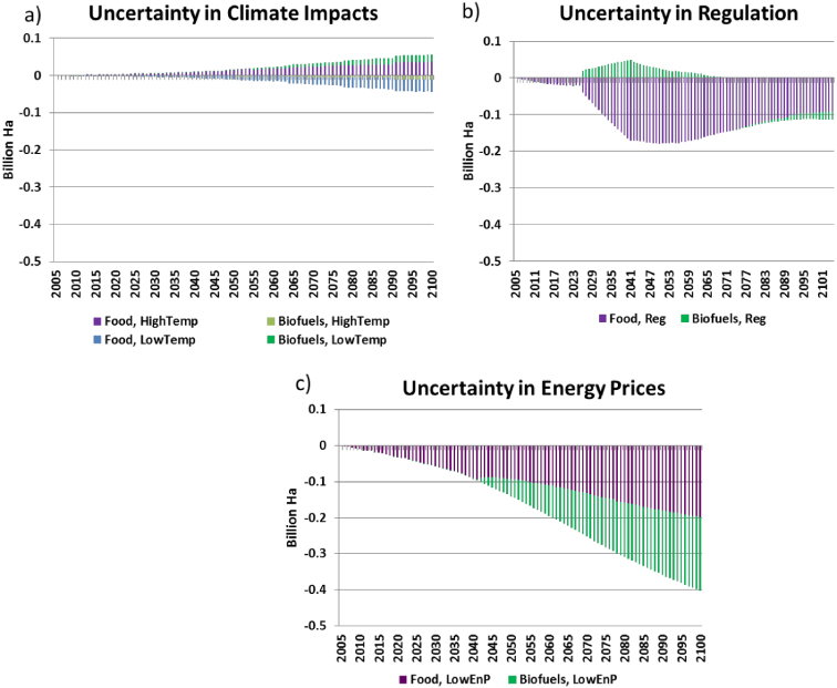
Figure 4. Land use changes relative to baseline under uncertainty in (a) climate impact, (b) GHG regulation, and (c) energy price scenarios as per figure 2.
Download figure:
Standard imageIntroduction of a land use GHG emissions constraint redirects land resources from food consumption towards climate abatement sectors, such as forestry and second-generation biofuels. After the GHG constraint is introduced, crop land declines considerably, while the area dedicated to biofuels' crops and feed stocks expands. Compared to the baseline scenario, cropland area is 180 MHa, or 10%, lower in 2050, whereas the land area dedicated to biofuels increases by 25 MHa, or by 43%, by 2050. Because net land-based GHG emissions are falling in the baseline scenario, in the long-run the GHG emissions constraint becomes less binding, requiring a lesser contraction of cropland and expansion of biofuels' feed stocks in 2100, relative to baseline. Cropland area declines by 95 MHa, or by 6.5%, whereas the land area dedicated to biofuels decreases by 20 MHa, or by 10%, by 2100. Overall, uncertainty in regulation results in variation of land use change of about 205 MHa by mid-century and about half that (115 MHa) in 2100 (figure 4(b)).
Oil and natural gas prices affect land use through three different channels. First, natural gas prices are closely linked to the costs of nitrogen fertilizers [30]. Previous studies, which found that intensive use of fertilizers can save land [50] have simply assumed that fertilizer use is exogenously specified. However, intensification is an endogenous phenomenon. Lower energy prices result in greater use of fertilizers and the contraction of cropland required for food and biofuel feedstocks. A second channel for energy impacts on land use arises due to the competition of biofuels with petroleum products as a fuel in the transportation sector. Indeed, oil prices are a key factor affecting competitiveness of biofuels in the long-run [28, 29]. Lower oil prices result in smaller demand for biofuels, and contraction of land dedicated to biofuels. Finally, there is a third, indirect channel through which energy prices affect land use decisions. This entails substitution in consumer demand towards sectors that benefit from lower oil prices.
Based on the model results, lower energy prices lead to a considerable decline in both cropland, and the land dedicated to biofuels. Compared to the baseline scenario, cropland area in 2100 declines by 200 million hectares, or 14%, and land area dedicated to biofuels decreases by 205 MHa, virtually eliminating the production of feedstocks in 2100 under the low energy price scenario. Overall, uncertainty in energy prices results in variation of land use change of 400 MHa (figure 4(c)), a figure, which is considerably higher than the variations due to climate impacts and policy uncertainty.
3.3. GHG emissions sensitivities
Figure 5 reports uncertainty in land-based GHG emissions (biofuels' offsets, afforestation and forest management, reduced deforestation, and use of fertilizers) owing to uncertainty in climate impacts, climate policy and energy prices. Figure 5(a) shows that climate impacts have a very modest effect on GHG emissions.
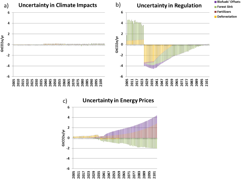
Figure 5. Change in land-based GHG emissions relative to baseline under uncertainty in (a) climate impact (HighTemp), (b) regulation, and (c) energy prices.
Download figure:
Standard imageDeclining food crop yields from higher temperatures result in an increase in GHG emissions from more use of fertilizers, increased deforestation, reduced afforestation, and smaller biofuels' offsets due to decreased consumption of first-generation biofuels. Overall, higher temperatures increase land-based GHG emissions by just 18 MtCO2e yr−1 relative to the baseline scenario in 2100.
By design, introduction of the GHG emissions constraint has a dramatic impact on the profile of emissions throughout the twenty first century. Relative to baseline, land-based emissions jump by a cumulative 85 GtCO2e in the 20 years prior to implementation of the regulation. This is due to investor anticipation of this impending regulation. Deforestation rates rise, and forest management focuses on near-term gains at the expense of longer term carbon stocks. Following implementation of the GHG regulation in 2025, natural land conversion ceases altogether, and forest managers begin focusing on growth in carbon stocks, at the expense of commercial output [51]. Fertilizer use and biofuels production also decline in the wake of the GHG emissions constraint which make these activities more costly. Overall, in the period: 2025–100, GHG emissions from land use cumulatively decline by 260 GtCO2e, with the constraint becoming non-binding at the end of this period. The resulting intertemporal leakage (the ratio of cumulative increase in GHG emissions preceding the GHG target to cumulative decline after the GHG target) is 33%.
As with land use, energy prices affect GHG emissions through several channels. First, lower energy prices imply smaller requirements for crops and biofuels' feed stocks, and correspondingly decrease GHG emissions caused by conversion of natural and managed forest areas for agricultural purposes. Second, lower energy prices decrease fertilizer production costs, thereby leading to increased usage and greater nitrous oxide emissions. Finally, lower energy prices result in greater consumption of petroleum products and depress petroleum displacement by biofuels, thus increasing the GHG emissions from liquid fuel combustion. The latter two effects appear to be more significant in the long-term context of lower energy prices. Compared to the baseline, annual GHG emissions flows from reduced biofuels' offsets (1.5 GtCO2e yr−1) and increased use of fertilizers (2.5 GtCO2e yr−1) due to lower energy prices in 2100, dominate the increase in forest sequestration (2 GtCO2e yr−1 ), resulting in a net increase of 2 GtCO2e yr−1 of GHG emissions (figure 5(c)).
4. Discussion
We find that variations in long-term energy prices have a profound impact on the optimal dynamic path of agricultural land use for food crops and biofuel feed stocks. However, as with most new methodological developments, introducing this intertemporal dimension into the model comes at a cost; as a consequence we are not yet able to offer the kind of geographic coverage which is customary in the land-based integrated assessment models [52–54]. Instead, we are forced to consider the competition for land use in food, fuel, forest products and ecosystem services at global scale. This necessarily limits our ability to speak to the heterogeneous impacts of climate change and the potential for geographic shifting of production in order to take advantage of changing climate [55]. Accounting for such shifts would further moderate the impact of adverse climate change on global land use, thereby strengthening our main finding. Disaggregation of the world's land resources would also allow for study of the role of local institutions and property rights in shaping the evolution of land use [56, 57]. Over the period of a century, such institutions are likely subject to change in the face of changing economic incentives, and these incentives are well captured in this long-run economic model.
Another important limitation of this work is the absence of a livestock sector in our model. Livestock production is an important source of GHG emissions [58], ruminant livestock compete for land with cropping and forestry, and intensive livestock production absorbs a large share of crop output, which we have subsumed into the composite food-processing sector [2, 59, 60]. Changing dietary preferences towards higher value foods, like meat and milk, due to an increase in global per capita income, will thus likely result in additional cropland expansion relative to our model baseline. The impact of climate change on livestock production is ambiguous, with temperature increases tending to favor small animals [61]. However, it is clear that GHG regulation would curtail growth in livestock consumption, suggesting that our analysis may understate the impact of GHG regulation on land use. Future work should introduce livestock activity explicitly into this framework.
Despite these important limitations, the framework outlined here has the capacity to deliver new insights about the long-run evolution of land use at global scale. Our model suggests that long-term uncertainty in energy price forecasts translates into variation in land use change of as much as 400 MHa. This is four times higher compared to variation in land use change from uncertainty in climate impacts on agricultural yields, and two times higher compared to maximum variation in land use change from uncertainty in GHG emissions targets. The economic response of indirect land use change with respect to energy prices involves complex linkages. Natural gas prices affect the use of fertilizers, which trigger endogenous response by land intensification. Oil prices are a key long-run determinant of biofuel demand, and higher oil prices result in significant requirements for land used in biofuels' feed stocks. Energy prices also indirectly affect land use decisions by shifting consumption between land-based goods and services and other sectors of the economy.
While the relatively smaller land use effects of climate change impacts can be explained by the modest yield effects due to climate change, the result that energy price uncertainty dominates GHG emissions regulation is not so obvious. This finding can be explained by two factors. First, the long-run effectiveness of the GHG emissions target is diluted by intertemporal substitution of land resources, the phenomenon known as 'green paradox' [62]. Secondly, our model baseline predicts a declining path of optimal land-based GHG emissions, due to slowing population growth, improving technology, and evolving consumer demands for food. This diminishes necessary changes in land use, as land becomes GHG neutral in the long-run.
It is important to consider whether this study may have overstated the range of possible energy prices in 2100—thereby skewing the findings in favor of energy price uncertainty. Towards this end, consider the evolution of oil price forecasts over the past decade. In 2003, EIA forecasts for oil prices in the year 2025 ranged from $17 to $35 [63]. By 2006, AEO forecasts for this same year had jumped to the range of $35–$95 [64], and by 2012 this range had expanded to $59–$193 [35]. In short, even as the duration of the forecast was cut in half, the range of uncertainty increased by a factor of seven! Energy prices are indeed highly uncertain.
Another robustness check involves asking the question: how much could we reduce the oil price uncertainty range in 2100, while still preserving the result that this source of uncertainty has a greater effect than that of climate impacts or climate policy. In this case, we find that if we allow baseline oil prices to rise more slowly, reaching $240/bbl in 2100, this source of uncertainty (i.e. $240 versus $60/bbl in 2100) remains equally important as a determinant of land use change uncertainty as is climate policy—and it is still much more significant source of land use change than climate impact uncertainty. This leads us to conclude that the link between energy prices and global land use change and GHG emissions is indeed worthy of greater attention in the future.
Acknowledgments
The authors thank Joshua Elliott for providing us DSSAT crop yield simulation data, David Lobell, and two anonymous reviewers for insightful comments and suggestions. We appreciate the financial support from the National Science Foundation, grant 0951576 'DMUU: Center for Robust Decision Making on Climate and Energy Policy'. IOP Publishing acknowledges that the article was produced with funding from the US Government and the author's obligation to give the US Government non-exclusive use of the article to the extent required under the US Government award.
Footnotes
- 3
We do not consider cellulosic-based ethanol here due to the difficulty of fitting additional ethanol in under the 'blend wall' in economies lacking flex fuel vehicles [28].
- 4
Ecosystem services are difficult to define, and it is even more difficult to characterize their production process [65]. This stems from several features, including: (a) the significant heterogeneity in ecosystem services, (b) the lack of markets and market prices, and (c) significant differences in definitions and modeling approaches in the economic and ecological literatures. While addressing these limitations is beyond the scope of this study, given their important role in the evolution of the long-run demand for land, we incorporate ecosystem services, albeit in a stylized fashion, into the global land use model for determining the optimal dynamic path of land use in the coming century. Further details on calculating ecosystem services are available in model's technical documentation [32].