

Abstract
Urban population now exceeds rural population globally, and 60–80% of global energy consumption by households, businesses, transportation, and industry occurs in urban areas. There is growing evidence that built-up infrastructure contributes to carbon emissions inertia, and that investments in infrastructure today have delayed climate cost in the future. Although the United Nations statistics include data on urban population by country and select urban agglomerations, there are no empirical data on built-up infrastructure for a large sample of cities. Here we present the first study to examine changes in the structure of the world's largest cities from 1999 to 2009. Combining data from two space-borne sensors—backscatter power (PR) from NASA's SeaWinds microwave scatterometer, and nighttime lights (NL) from NOAA's defense meteorological satellite program/operational linescan system (DMSP/OLS)—we report large increases in built-up infrastructure stock worldwide and show that cities are expanding both outward and upward. Our results reveal previously undocumented recent and rapid changes in urban areas worldwide that reflect pronounced shifts in the form and structure of cities. Increases in built-up infrastructure are highest in East Asian cities, with Chinese cities rapidly expanding their material infrastructure stock in both height and extent. In contrast, Indian cities are primarily building out and not increasing in verticality. This new dataset will help characterize the structure and form of cities, and ultimately improve our understanding of how cities affect regional-to-global energy use and greenhouse gas emissions.
Export citation and abstract BibTeX RIS

Content from this work may be used under the terms of the Creative Commons Attribution 3.0 licence. Any further distribution of this work must maintain attribution to the author(s) and the title of the work, journal citation and DOI.
1. Introduction
Urban areas occupy only a very small fraction of the Earth's land area [1], house half of human population [2], consume 60–80% of final energy [3], and concentrate materials, wealth, and innovation [4, 5]. Urban landscapes influence local-to-regional climate, hydrology, habitat and biodiversity, agricultural and forested lands, and biogeochemical cycles [6–8]. Global urban population is projected to increase by 1.8 billion from 2000 to 2025. The majority of this increase (1.1 billion) will be in cities with >1 M inhabitants, and both the number and population of mega-cities (>10 M inhabitants) are projected to more than double (table S1 available at stacks.iop.org/ERL/8/024004/mmedia) [2]. While recent trends toward a more urbanized global population are well-established, global-scale information and understanding of other dimensions of urban change, such as the physical characteristics, is poor [9]. Urban form and structure are key factors that determine urban energy use and emissions [10], and urbanization fundamentally changes the 2- and 3-dimensional form and structure of cities, including the number of buildings, their geometry, size, volume, proximity, and density.
Global mapping of urban land use generally relies on remote sensing data, often in combination with gridded population data, and focuses almost exclusively on urban extent [11]. Sensors used for this purpose include ESA's SPOT4 VEGETATION [12]; ESA's medium resolution imaging spectrometer (MERIS) [13]; NOAA's defense meteorological satellite program/operational linescan system (DMSP/OLS) sensors [14]; and NASA's moderate resolution imaging spectroradiometer (MODIS) [15]. DMSP/OLS sensors have been used to map economic activity [16] and urban change at coarse scales [17]. Two recent studies have documented changes in the global urban footprint [1, 18]. However, no study to date has examined changes in both extent and structure of urban built environments globally.
Built environments contain numerous efficient microwave backscattering surfaces, and microwave remote sensing can therefore be used to characterize urban areas [19–21]. Orbiting microwave scatterometers are active remote sensing instruments that measure the microwave power scattered back to the instrument from the Earth's surface, with frequent global coverage at relatively coarse spatial resolution. Space-borne scatterometry has been used primarily to quantify surface wind vectors over the ocean [22], but early analyses of data from NASA's NSCAT Scatterometer mission revealed a pronounced backscatter signature from major urban areas [23]. More recent analysis using NASA's SeaWinds scatterometer data demonstrate that centers of large cities (scale length ∼5–10 km) have very high backscatter returns, with backscatter power return dropping by roughly 50% in suburban areas, and even more in rural outskirts of cities [21].
In this paper, we examine spatio-temporal patterns in global urban extent and form by analyzing 11 years of SeaWinds microwave backscatter power return (PR) data in combination with DMSP/OLS nighttime lights (NL). Our results show previously undocumented recent and rapid changes in urban areas worldwide during 1999–2009 that reflect pronounced shifts in urban form and structure.
2. Data sets and methods
We analyzed data from two space-borne sensors—mean summer backscatter power ratio (PR) from NASA's SeaWinds microwave scatterometer (Ku-band, 13.4 GHz) [24], and mean annual stable nighttime lights (NL) from DMSP/OLS [25, 26]—to quantify and classify changes in characteristics of urban agglomerations from 1999–2009. Because these data sets are at different spatial resolutions, we re-processed each to have a common 0.05° spatial resolution, approximately equivalent to the coarsest data set—PR. Our analysis focused on larger cities and urban agglomerations identified in two stages: (i) we extracted 11 × 11 and 21 × 21 grids of 0.05° cells centered on 100 large cities, and (ii) we masked out non-urban land globally by excluding all 0.05° cells with less than 20% urban land use, based on a MODIS-derived map of global urban land extent in 2001 at 500 m spatial resolution [15]. To evaluate the ability of microwave backscatter to capture macro-scale urban change across a range of urbanization levels, we aggregated 1999–2009 PR increases to provincial values in China by area-weighted summing of PR increase for all grid cells with urban cover ≥20% within each province, and compared this to provincial increase in residential floor area. Finally, we used a k-means cluster analysis to classify these 35 359 urban grid cells (∼830 000 km2), based on 1999 PR and NL (initial state) and their changes from 1999 to 2009. Data sets and methods are described in more detail in the Appendix.
3. Results
Urban backscatter increases in China are strongly correlated with increases in provincial residential floor area (figure 1), which represents ∼70–80% of new floor space completed in China between 1999 and 2009 [27, 28]. Residential floor area strongly correlates with residential building surface area and volume. Differences in developmental stage of urbanization likely contribute to the variation in this relationship. For example, cities in Guangdong, Shanghai and Beijing were among the first to transform their urban housing market from a centrally planned system to a market-oriented one [29, 30]. They were among the first to construct new central business districts and have now reached a more mature stage of urbanization. With commercial real estate on the rise in these cities, residential construction will represent a smaller fraction of total building construction.
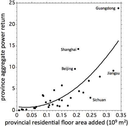
Figure 1. Relationship between 1999 to 2009 change in residential floor area and grid cell area-weighted aggregate backscatter power-ratio return (PR) for China's 22 mainland provinces, 4 municipalities, and 5 autonomous regions, including only 0.05° grid cells with urban cover ≥20%. Solid line is best-fit polynomial regression (y = 0.83 − 9.7x + 160x2;R2 = 0.64).
Download figure:
Standard imageLarge urban agglomerations displayed a wide range of changes in nighttime lights and urban backscatter (figures 2(a)–(l)). For example, structural backscatter was essentially constant in Kinshasa (figure 2(k)), a city that experienced high population growth over the last decade but where urban growth is largely driven by the informal economy [31] and is characterized by unplanned developments and slums on the outskirts of the city [32]. Large increases in structural backscatter occurred in Shanghai (figure 2(f)), where the number of high-rise buildings (>30 m) quadrupled from 1999 to 2006 [33]. Perhaps most significantly, there was a remarkable contrast in urban change between mega-cities in East Asia and South Asia, e.g., Beijing and Shanghai contrasted with Delhi and Dhaka (figures 2(e)–(h)).
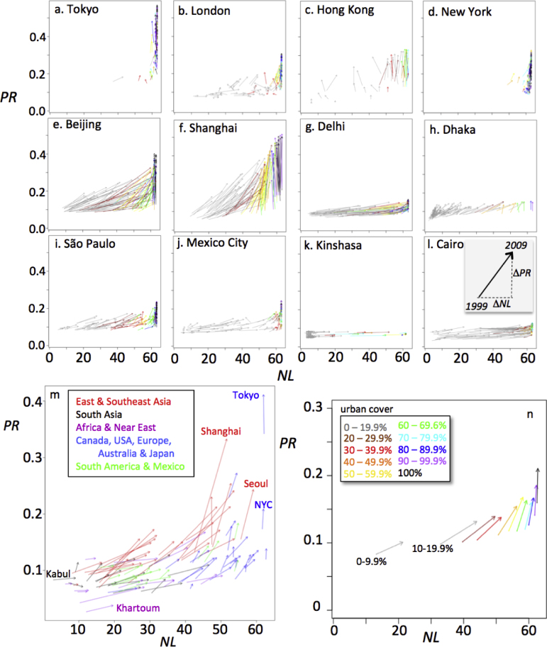
Figure 2. (a)–(l) Changes in structural backscatter (PR) and nighttime lights (NL), 1999–2009, for 12 large cities. Arrows represent non-water, 0.05° cells in an 11 × 11 grid around each city's center; tail and head are at 1999 and 2009 coordinates of cell PR and NL, respectively; horizontal change is increase (or decrease) in nighttime lights, and vertical change is increase (or decrease) in structural backscatter (see inset in panel l). Arrow color corresponds to per cent urban cover (see legend in panel n). (m) Aggregate mean change per city in structural backscatter and nighttime lights for 11 × 11 grids centered on 100 large cities (listed in supplementary table S2 available at stacks.iop.org/ERL/8/024004/mmedia). (n) Aggregate mean change in structural backscatter and nighttime lights for 11 × 11 grids, binned by urban cover, centered on 100 large cities. Note that urban cover <20% mask was not applied to these grids.
Download figure:
Standard imageIn the vicinity of the 100 large cities from six continents examined here (figure 2(m); listed in table S2 available at stacks.iop.org/ERL/8/024004/mmedia), increases in nighttime lights (NL) between 1999 and 2009 were inversely proportional to fractional urban cover in 2001, and were small to negligible for areas with urban cover >70% (figure 2(n)). This is consistent with an earlier study that the NL signal of urban change for large, rapidly developing cities emphasizes growth in the peri-urban region around an NL-stable urban core [17]. Increases in urban structural backscatter (PR) had little correlation with 2001 fractional urban cover, although aggregate backscatter increases were lower for cells with very low urban cover.
When the observed changes in global urban structural backscatter were stratified into bins according to different levels of nighttime lights in 1999, backscatter increase was largest where values of nighttime lights in 1999 were highest; this pattern was evident at both global and national scales (figure S1 available at stacks.iop.org/ERL/8/024004/mmedia). Cells with NL ≥ 60 in 1999 (i.e., already highly illuminated) accounted for 27% of urban grid cell area and 45% of the area-weighted aggregate increase in backscatter power return. Structural backscatter also increased in urban cells with NL < 60 in 1999, but changes were generally smaller, suggesting that the increase in built-up infrastructure was most pronounced in urban cores, where changes are most difficult to detect with optical remote sensing. In short, a unique and important value of these data are their ability to detect changes in urban 3-D structure which are unobservable with optical satellite data.
A k-means cluster analysis of NL and PR data yielded 5 overlapping classes (table 1, figure 3). Two clusters (Classes 3 and 4) include grid cells with low PR and NL in 1999 and low urban cover in 2001 (figures 3(b), (d) and (f)). These classes had the smallest increases in urban structural backscatter (figure 3(c)). Class 3—Rapid Lighting Growth with Little Structural Growth—had the largest increases in nighttime lights during 1999–2009 of any class, while nighttime lights generally decreased in Class 4—Slow (or No) Growth (figure 3(e)). These two classes occurred either at smaller cities (one to a few adjacent 0.05° grid cells), at the perimeter of large cities, or on corridors radiating out from or linking large cities. The other three classes were predominantly in large cities (usually 10–100+ contiguous 0.05° grid cells). Of these, Class 2 had the highest values of urban cover in 2001 and NL and PR in 1999 (figures 3(b), (d) and (g)). Class 1—Rapid Structural Growth in Urban Core—had very large urban backscatter increases with small to moderate nighttime light increases, and occurred almost exclusively in large cities in China and South Korea. Class 2—Moderate Structural Growth in Urban Core—had moderate urban structure increases but no changes in nighttime lights. This type of change occurred in the core of large cities in North America, Europe, Japan, and, to a limited extent, in South Asia, South America, and South Africa. Class 5—Slow/Moderate Growth/Infilling—had small increases in urban structure with negligible to small decreases in nighttime lights (figures 3(c), (e)); this class was the dominant urban class in North America, Europe, and in large cities in India, but was not common in China. See the supplemental material (available at stacks.iop.org/ERL/8/024004/mmedia) for regional k-means class maps.
Table 1. Urban change classes for 0.05° grid cells with urban covera ≥20% (see figure 3 for class distributions, and supplementary figure S2(a)–(f) (available at stacks.iop.org/ERL/8/024004/mmedia) for mapping of classes).
| Urban class | #cells | Initial state | Change | Description | |||
|---|---|---|---|---|---|---|---|
| Urban% | NL1999 | PR1999 | ΔPR | ΔNL | |||
| 1 | 636 | Moderate | High | High | Very high | Moderate | Rapid structural growth in urban core |
| 2 | 2 015 | High | Very high | Very high | Moderate | Nil | Moderate structural growth in urban core |
| 3 | 6 639 | Low | Low | Low | Low | High | Large increase in lighting, little structural growth |
| 4 | 12 695 | Low | Low | Low | Very low | Low (<0) | Decrease in lighting; little (or no) structural growth |
| 5 | 13 410 | Moderate | High | Moderate | Low | Low/nil | Slow/moderate infilling or structural growth |
aUrban per cent cover c. 2001 from MODIS [15].

Figure 3. A k-means cluster analysis of grid cells with urban cover ≥20% generated 5 classes: (a) global distribution of 35 359 grid cells by class in ΔNL − ΔPR space. (b–f) Boxplots summarizing the distribution of data for each class: (b) urban per cent cover c.2001, (c) ΔPR, (d) PR in 1999, (e) ΔNL, and (f) NL in 1999. Boxes show the inter-quartile range (i.e., 50% of the data centered on the median); notches in boxes provide approximate 95% confidence intervals on the median; whiskers (outer lines) extend to smaller of extreme value or 1.5 times the length of the inter-quartile range above and below the median. Outliers (i.e., those points outside of the whiskers) have been omitted. Also see table 1.
Download figure:
Standard imageDramatic differences between urban development in China and India are apparent in the time series of urban backscatter and nighttime lights. To illustrate, we focus on the two largest cities in China and India: Beijing (15 M residents in 2010; [2]), Shanghai (20 M), Delhi (22 M), and Mumbai (19 M) (figure 4). In all four cities, nighttime light values in the city core were high and constant (saturated) from 1999 to 2009; this core spans ∼20 km. Nighttime light values increased substantially over the decade around the urban core in Shanghai, Beijing, and Delhi, but much less so in Mumbai. Corridors of development radiating out from the city center are also evident in the nighttime lights data. Zhang and Seto [17] identified similar changes in nighttime lights, 1992–2007, for the lower Yangtze and Pearl River regions in China. Large increases in urban structural backscatter occurred only in the urban cores of Shanghai and Beijing (figure 4). Moderate structural backscatter increases also occurred west of Shanghai's core. Structural backscatter increases in Delhi and Mumbai, on the other hand, were small and restricted to the urban core (figure 4). The nighttime light increases around the urban cores of the capitol cities of Delhi and Beijing were similar in scale and magnitude, while the backscatter increases in their urban cores were very different.

Figure 4. Plan view maps of 21 × 21 grids of 0.05° grid cells centered on Beijing and Shanghai, China; and Delhi and Mumbai, India. Each small graph has an 11-year time series of (left column) mean annual DMSP/OLS NL or (right column) mean summer SeaWinds PR for all non-water 0.05° grid cells (see samples at top of figure). Color of points in each grid cell time series is determined by the magnitude of the slope of a linear trend fit to 11 years of annual PR or NL data. The urban core of each city had high and constant (dark blue) nighttime light (NL) values, while the periphery often had low and constant (dark blue) nighttime light values. Large changes in nighttime lights occurred in the periphery of the city core or in corridors radiating from the city core. In contrast, increases in urban structural backscatter (PR) were highest in the city core in all cities; these increases were small in Delhi and Mumbai, and large in Beijing and Shanghai. Note that urban cover <20% mask was not applied to these grids; blanks are open water.
Download figure:
Standard image4. Discussion and conclusions
DMSP/OLS nighttime lights and SeaWinds microwave backscatter provide complementary information related to the physical dimensions of urban change. DMSP/OLS passive sensing of emitted light at night has been studied for decades, and provides a metric of urban extent that is correlated with metrics of urban activity such as economic activity and electricity use [14, 16, 17, 34–36]. Our use of SeaWinds active backscatter is a new application of an established remote sensing technology. Microwave backscatter return from Earth surfaces is a function of wavelength and surface properties—roughness, orientation, and dielectric properties (i.e., vegetation and soil moisture, building materials) [37]. At SeaWinds' spatial resolution, backscattered power reflects the aggregate character of the land surface—including both vegetation and the built-up environment—over ∼10 km. Seasonal variation in SeaWinds backscatter can arise from moisture changes or freeze thaw [38, 39], but a large temporal increase over a decade, detected by a stable instrument, can only result from a temporal trend in land surface properties (e.g., reforestation [40], or development in built-up infrastructure). We infer that the significant backscatter increase in major cities around the world, and particularly in the centers of these cities (see figures 2, 4, and S1 available at stacks.iop.org/ERL/8/024004/mmedia), is caused by changes in the built environment, not urban afforestation. This follows from previous studies with MODIS normalized-difference vegetation index (NDVI) and DMSP/OLS data that show there is relatively little vegetation in the centers of urban areas [41]. We also infer that these changes in built-up infrastructure are related to building volume (height and density). This inference is supported by the relationship between backscatter change and residential floor area change in China and by the very different backscatter changes between large cities in China and large cities in India, where there is strong evidence of differences in verticality of building development (discussed below).
Examination of urban backscatter and nighttime lights data for 100 large cities indicates a general trajectory in urban development at the scale of tens of kilometers (figure 2(m)). Large urban agglomerations with low initial light intensity and urban structural backscatter were more likely to have larger nighttime light increases than backscatter increases, while agglomerations with high light intensity showed larger increases in backscatter than nighttime lights. Intermediate urban areas tended to have increases in both. Only one city of the 100 examined—Kanpur (Cawnpore), India—showed an aggregate (11 × 11 grid mean) decrease in urban backscatter. Chinese cities accounted for nine of the ten urban agglomerations with the largest area-weighted mean backscatter increase; Seoul had the 8th largest increase. Bangalore had the largest backscatter increase of an Indian city, with about 13% of the increase of Shanghai. Chinese cities accounted for seven of the ten urban agglomerations with the largest area-weighted mean nighttime light increase, with Luanda, Ho Chi Minh City, and Lagos ranking 1st, 3rd, and 8th. The Indian cities of Chennai (Madras), Hyderabad, Delhi, and Bangalore ranked 12th–15th, with about 60% of the increase of Luanda. Note that since the DMSP/OLS sensors saturate, cities with relatively low light levels in 1999, like Luanda, had the greatest potential for increase.
The tremendous increase in the verticality of built-up infrastructure in Chinese cities over the past decade (figure 2(m)) is a function of several factors: severely constrained land markets from 1949 to 1978, post-reform introduction of a land and real estate market, and the subsequent skyrocketing in land prices [42]; dramatic increases in urban market housing prices, in part due to an increase in urban population and decline in the importance of the household registration system [43, 44]; local officials acting as land developers and driving up urban land markets and land speculation [45]; large-scale investments in transport infrastructure in China's cities [46]; and land use and zoning laws [47], including building height restrictions (or lack thereof) in many Chinese cities [48].
The k-means cluster analysis identified broad classes of urban dynamics based on changes in nighttime lights and microwave backscatter over a 10-year period. The analysis was limited to grid cells with urban cover ≥20% in 2001, and so did not include grids cells that became significantly urbanized after 2001 (see gray arrows in figure 2, and background image of 2009 nighttime lights in supplemental figure S2(a)–(f) available at stacks.iop.org/ERL/8/024004/mmedia). The significant global sample of classified grid cells (∼840 000 km2), which included large- and moderate-sized cities on all continents, revealed clear geographic patterns worldwide that reflect regional differences in urban dynamics between 1999 and 2009 (see supplemental figure S2), including striking differences between cities in the highly populated and rapidly developing countries of China and India.
Two important factors that explain the expansive but not vertical growth of India's cities are the large informal market for land and housing [49] combined with restrictive land use controls on floor area ratio and urban land ceiling [50]. Land use controls have led to excessive, low density, leapfrog development across India's cities, and a marked lack of a densely built-up urban core [51]. The high level of informality is pervasive not only in land and housing markets, but also in the planning system, which has led to inadequate infrastructure investments [52].
It is important to note that neither the eponymously named SeaWinds nor the DMSP/OLS sensors were designed to measure or monitor urban dynamics. Sensor saturation limits the utility of NL data for studying changes at the core of highly urbanized areas [17]. Coarse resolution SeaWinds data cannot detect small cities [21], nor resolve spatial details of structural change in large cities. The day/night band on the visible infrared imaging radiometer suite (VIIRS), launched in October 2011, will provide improved remote sensing of some components of future urban change [53]. However, cities, especially those in the developing world, have been changing rapidly—global urban population grew by ∼700 million in the past decade [2]—and more comprehensive information about recent urban change will help us understand and predict how cities will change in the future.
Reliable, global information on how cities are changing will become increasingly important as populations become increasingly urban [54]. Urbanization involves simultaneous economic, demographic, and land cover change: economic transition from agriculture to industry/services; increased concentration and clustering of population in urban areas; loss of natural ecological systems to a built environment; and increasing building density within existing urban areas. Global characterization of urbanization requires adequate datasets in all three dimensions. Demographic and economic data are available from national and international statistical data repositories (e.g., census data), and global urban land cover data has primarily focused on extent. The global urban backscatter dataset that we explore here provides new information that is diagnostic of urban change (building density and volume) and that should be useful for examining development trajectories in the context of land use controls and their histories, governance and institutions, and economic development. Further, synthesis of urban backscatter data with population data and economic data has the potential to yield new ways to identify and characterize previously undocumented types of urbanization and changes in cities. More generally, integration of diverse remote sensing and socio-economic datasets has the potential to enable new applications, including visualization of climate change mitigation and adaptation challenges for different urban areas, evaluation and comparison of the underlying urban structure and form, and the relationships among urban structural properties, greenhouse gas emissions, and climate change vulnerability across a range of urban settlement types and geographies. Although this study has focused primarily on the world's largest cities, the methodology presented has the potential to be applied to cities worldwide, though more work is required to better understand the limits of the scatterometer data for smaller urban areas.
Acknowledgments
This work was supported by grants from NASA (NNX08AE59G, NNX10AP11G, NNX11AE75G, NNX12AM82G, NNX11AE88G) and NSF (EAR-1038818). We thank D Long for comments and for developing the scatterometer database (www.scp.byu.edu), K Anlar and J Boyko at CEIC-US for providing the China provincial residential floor area data, J Gray and S Glidden for help with the figures, and two anonymous reviewers for comments on an earlier draft. The authors have no conflicts of interest related to this research.
Appendix.: Data sets and methods
A.1. SeaWinds microwave backscatter
The SeaWinds scatterometer (Ku-band, 13.4 GHz) operated from July 1999 to November 2009. SeaWinds backscatter data ( in dB) are available globally from July 1999 through November 2009 from the NASA scatterometer climate record pathfinder (SCP) project [24]. The native sensor resolution is approximately 25 km, with near daily repeat frequency. SCP data processing combines multiple orbit passes to generate image products with improved spatial and reduced temporal resolution [55]. For the analysis reported here we used the 'quev' product, which is derived from vertical polarization (54° incidence angle), combined morning and afternoon overpass data, yielding 4-day composites at 4.45 km nominal spatial resolution. Analysis with horizontal polarization (46° incidence), combined overpass data generated very similar results and are not reported here. SeaWinds data are available at www.scp.byu.edu.
We used Delaunay triangular interpolation to re-project the 4-day composite data to 0.05° lat.-long. To minimize variability introduced by transient non-construction events that affect backscatter returns (e.g., weather) and to avoid winter freeze-thaw signals, we generated for each calendar year a 3-month average (July–September north of 23°S, January–March south of 23°S) by first converting backscatter from decibels (dB) to the power-return-ratio or  , and then averaging PR over all 4-day composites in each 3-month period. SeaWinds backscatter has been shown to be insensitive to a small city (∼8000 people), even when processed for enhanced spatial resolution [21].
To aggregate PR to China provincial values for comparison with provincial residential floor area data (see below), we assigned each 0.05° grid cell in China to a province, using the GADM global administrative boundary map (v.2; www.gadm.org). We then excluded grid cells with urban cover <20% (see below) and summed PR over the remaining grid cells (ΣPR), weighting the terms in the sum by relative grid cell area. The provincial change in backscattered microwave power, ΣPR2009 minus ΣPR1999, was correlated with the increase in provincial residential floor area.
A.2. DMSP/OLS stable nighttime lights
NOAA has generated gridded maps at 30'' resolution (∼1 km) of annual stable nighttime lights [25, 26]. The OLS sensors collect 6-bit data recorded as digital number (integer) values that range from 0 to 63. We used NOAA's calibration by quadratic polynomial fit to intercalibrate between sensors [56], using the calibration parameters for stable nighttime lights, and selecting the sensor with the best polynomial fit in years with data from multiple sensors—OLS sensor F12 for 1999, F14 for 2000–2001, F15 for 2002–2003, and F16 for 2004–2009 [57]. The NL data set has been shown to be correlated with urban population, and can detect small cities with populations of <1000 in developed countries [26]. These gridded NL maps were aggregated to 0.05° spatial resolution by taking the average of NL digital number values in each 0.05° cell. Annual NL data are available at www.ngdc.noaa.gov/dmsp/downloadV4composites.html.
A.3. MODIS global urban extent
To restrict global analysis to urban areas, we used the map of Global Urban Extent at 500 m resolution, derived from a supervised classification of MODIS surface reflectance data [15]. Dominant cover (>50%) of MODIS urban pixels is non-vegetated and composed of human-constructed elements such as buildings and roads. We computed urban per cent cover at 0.05° resolution as the per cent of urban 500 m pixels in each 0.05° grid cell, and defined a rural mask as urban cover <20%. MODIS Global Urban Extent data are available at www.sage.wisc.edu/people/schneider/research/data.html.
A.4. k-means cluster analysis
k-means cluster analysis [58] was done with the kmeans clustering algorithm in R (version 2.14.2; www.r-project.org/). Clustering used 4 input variables (NL1999, PR1999, ΔNL, ΔPR), to capture both grid cell initial state (1999) and change in state (1999–2009). The number of clusters was selected based on inspection of within-group sum of squares, and by visualizing resulting clusters in ΔNL and ΔPR space.
A.5. China residential floor area
Monthly year-to-date provincial data for residential floor area (completed and under construction) are collected by the Chinese National Bureau of Statistics. Data were downloaded from the CEIC online database (www.ceicdata.com; July 2012). We calculated the 1999–2009 increase in residential floor area as the sum of December year-to-date area completed for 1999 through 2008, plus the July 2009 (year-to-date) area under construction.