

Abstract
Glacial isostatic adjustment (GIA) represents a source of uncertainty for ice sheet mass balance estimates from the Gravity Recovery and Climate Experiment (GRACE) time-variable gravity measurements. We evaluate Greenland GIA corrections from Simpson et al (2009 Quat. Sci. Rev. 28 1631–57), A et al (2013 Geophys. J. Int. 192 557–72) and Wu et al (2010 Nature Geosci. 3 642–6) by comparing the spatial patterns of GRACE-derived ice mass trends calculated using the three corrections with volume changes from ICESat (Ice, Cloud, and land Elevation Satellite) and OIB (Operation IceBridge) altimetry missions, and surface mass balance products from the Regional Atmospheric Climate Model (RACMO). During the period September 2003–August 2011, GRACE ice mass changes obtained using the Simpson et al (2009 Quat. Sci. Rev. 28 1631–57) and A et al (2013 Geophys. J. Int. 192 557–72) GIA corrections yield similar spatial patterns and amplitudes, and are consistent with altimetry observations and surface mass balance data. The two GRACE estimates agree within 2% on average over the entire ice sheet, and better than 15% in four subdivisions of Greenland. The third GRACE estimate corrected using the (Wu et al 2010 Nature Geosci. 3 642–6)) GIA shows similar spatial patterns, but produces an average ice mass loss for the entire ice sheet that is 64 − 67 Gt yr−1 smaller. In the Northeast the recovered ice mass change is 46–49 Gt yr−1 (245–270%) more positive than that deduced from the other two corrections. By comparing the spatial and temporal variability of the GRACE estimates with trends of volume changes from altimetry and surface mass balance from RACMO, we show that the Wu et al (2010 Nature Geosci. 3 642–6) correction leads to a large mass increase in the Northeast that is inconsistent with independent observations.
Export citation and abstract BibTeX RIS

Content from this work may be used under the terms of the Creative Commons Attribution 3.0 licence. Any further distribution of this work must maintain attribution to the author(s) and the title of the work, journal citation and DOI.
1. Introduction
Over the past 20 years, the mass balance of the Greenland Ice Sheet (GrIS) has been increasingly negative, driven by changes in both the surface mass balance (SMB), and ice dynamics (Rignot et al 2011, Velicogna 2009, Khan et al 2010, Pritchard et al 2009, van den Broeke et al 2009). Mass losses from the GrIS are significant contributors to global sea level rise and freshwater fluxes to the North Atlantic (Rignot et al 2011, Bamber et al 2012).
Time-variable gravity measurements from the GravityRecovery and Climate Experiment (GRACE) provide a powerful tool for estimating monthly ice sheet mass balance (Tapley 2004). To calculate ice mass balance the GRACE mass changes need to be corrected for glacial isostatic adjustment (GIA), i.e. the mass change associated to the Earth's ongoing viscoelastic response to the redistribution of ice and water masses that have occurred following the last deglaciation. GIA is usually removed using a priori corrections (Wu et al 2010). In Antarctica, the GIA correction represents the largest source of uncertainty in the GRACE ice mass balance estimates (Ivins and James 2005, Velicogna 2006, Velicogna and Wahr 2013). In Greenland, the GIA correction averaged over the entire GrIS is much smaller than in Antarctica. Still, differences between published GIA corrections impact the GRACE ice mass estimates and associated accuracy, particularly at regional scale, where the GIA correction may locally represent a significant portion of the GRACE signal (Simpson et al 2009, Wu et al 2010, A et al 2013). Constraining GIA corrections at the regional level will help improve the overall accuracy of the GRACE ice mass estimates.
Uncertainties in GIA models come from a lack of constraints on global ice sheet history since the Last Glacial Maximum (LGM), and the Earth's internal rheological structure (Ivins and James 2005). There are two main classes of GIA models: (1) global (Peltier 2004) and (2) regional models (Ivins et al 2013). The regional models are constrained by local datasets, such as relative sea level, GPS measurements of crustal uplift, and geological records (Ivins and James 2005, Mackintosh et al 2011, Simpson et al 2011, Spada et al 2012). Wu et al (2010) derive an alternative global GIA estimate using an inverse method. Alternative regional GIA corrections have been calculated through a combination of ice mass balance estimates from satellite altimetry and gravimetry (Riva et al 2009, Gunter et al 2013). On average over the entire GrIS, the mass change corresponding to the Wu et al (2010) correction is 15 times larger than the other published GIA corrections, which yields an ice mass balance estimate much smaller than other published estimates. Prior GIA-evaluation studies compared GIA estimates to 3D ice sheet/bedrock models (Olaizola et al 2012), compared mass rates between GRACE and altimetry data (Gunter et al 2009), or evaluated the input data used to constrain the derivation of the GIA.
Here, we present a new methodology to evaluate GIA corrections over Greenland that compares the GRACE ice mass balance estimates with observations of surface mass balance (SMB) from the Regional Atmospheric Climate Model (RACMO) (Ettema et al 2010), and observations of ice volume change from ICESat and Operation IceBridge (OIB) laser altimetry data (Krabill et al 2002, Schenk and Csatho 2012, Zwally et al 2002). We evaluate the different GIA corrections by determining the level of compatibility of the GRACE estimates with the amplitude and spatial pattern of these independent observations. These three datasets are fundamentally different: GRACE measures total mass change, RACMO reconstructs surface mass balance that represents only a portion of the total ice mass change, as it does not account for the ice discharge, and altimetry measures ice volume change. Ice volume may be translated into mass change if the density at which elevation changes are taking place is known. In general, this density is not well known, which introduces large uncertainties (Zwally et al 2005). Here we choose not to convert the volume changes into mass, and note that elevation changes cannot be directly compared with mass changes. Surface elevation measurements have the advantage of a low sensitivity to GIA and high sensitivity to SMB.
We compare the three datasets during the period September 2003–August 2011. Within the period, we consider two sub-periods, September 2003–September 2007 and September 2007–August 2011, to separate the different sources of mass variability and identify uncertainties. The sub-periods are chosen based on the availability and sampling of the altimetry dataset. We use our approach to evaluate three GIA corrections: Simpson et al (2009), A et al (2013), Wu et al (2010). In the following sections we discuss how the comparison is implemented, how we use the results to evaluate different GIA corrections, and conclude on the robustness of the corrections.
2. Data and methodology
2.1. GRACE
We use 94 monthly GRACE Release-5 (RL05) gravity solutions provided by the Center for Space Research (CSR) at the University of Texas (Tapley et al 2004, Bettadpur 2012b) for the period September 2003–August 2011. This is the longest period for which all the examined datasets are available. GRACE RL05 data use improved dealiasing products of the Earth's non-tidal atmospheric and oceanic variations, updated background gravity models, and improved processing methods (Bettadpur 2012b). The dealiasing products remove non-tidal atmospheric and oceanic mass variability from the monthly GRACE products using outputs from the European Centre for Medium-Range Weather Forecasts (ECMWF) and the baroclinic Ocean Model for Circulation and Tides (OMCT) (Bettadpur 2012b) . A key improvement with the new release (RL05) data products is the marked reduction of 'striping' errors and spherical harmonic noise compared to the fourth release (RL04) (Bettadpur 2012a). Each CSR gravity field solution consists of fully normalized spherical harmonic Stokes coefficients, Cℓm and Sℓm up to degree, ℓ, and order, m, 60. C20 coefficients derived from GRACE show anomalously large variability due to excessive noise and high sensitivity to tidal aliasing errors (Chen and Wilson 2010). We replace the GRACE-derived C20 coefficients with monthly estimates from satellite laser ranging (SLR) (Cheng and Tapley 2004). GRACE does not recover degree-1 coefficients, which are related to motion of the Earth's geocenter (Swenson et al 2008). The omission of degree-1 can significantly degrade estimates of ice mass variability by excluding long-wavelength components of the Earth's mass change, and by leaking far-field signals into the regional estimates (Velicogna 2009). We account for the variation of degree-1 using coefficients calculated from a combination of GRACE coefficients and ocean model outputs (Swenson et al 2008).
We apply different GIA corrections: (1) Simpson et al (2009), (2) A et al (2013), and (3) Wu et al (2010), to the GRACE data and obtain three different ice mass balance estimates. For the remainder of the paper, we refer to the three corrections as SM09-GIA, AW13-GIA, and Wu10-GIA, respectively, and to the associated ice mass estimates (GRACE-GIA) as SM09, AW13, and Wu10. The SM09-GIA correction is a regional GIA model using a thermomechanical ice sheet model calibrated with relative sea level data and geological observations of ice sheet extent (Simpson et al 2009). The AW13-GIA correction is an update to the 2007 Paulson global GIA model (Paulson et al 2007) using the ICE-5G deglaciation history, compressibility parameters from the Preliminary Reference Earth Model (PREM), and a layered approximation of the Peltier VM2 mantle viscosity profile (A et al 2013). The Wu10-GIA correction is generated using a global inversion method including terrestrial and space geodetic data (GPS, satellite laser ranging, and very long baseline interferometry), and ocean bottom pressure output from the JPL ECCO model (Wu et al 2010).
Greenland ice mass anomalies are calculated relative to the period September 2003–August 2011. We account for the elastic deformation of the solid Earth induced by variations in mass loading using load Love numbers of gravitational potential, kℓ, calculated by Han and Wahr (1995) (Wahr et al 1995, 1998). We simultaneously fit annual and semiannual signals, a linear trend and a constant to the Stokes coefficient time series. To reduce the random spherical harmonic error component, which increases as a function of decreasing wavelength, we smooth the GRACE data using a normalized version of Jekeli's Gaussian averaging function with a 250 km radius (Jekeli 1981, Wahr et al 1998). Finally, we generate evenly spaced latitude–longitude grids for the three GRACE-derived ice mass changes (figure 1).
We use these maps to compare spatial patterns in the SM09, AW13, and Wu10 ice sheet mass changes. To evaluate how the three GIA corrections impact the ice mass balance estimates at a regional scale, we divide the ice sheet in four regions: Northwest (NW), Northeast (NE), Southwest (SW) and Southeast (SE) as shown in figure 1. For each region, we calculate the average time series using a least squares mascon approach (Tiwari et al 2009, Jacob et al 2012). Each of the four regions is composed of many small mascons. Each mascon is a 3-degree diameter equal-area spherical cap with a unit mass distributed uniformly on the mascon equal to 1 cm of water (Farrell 1972). For each mascon, we calculate a set of Stokes coefficients, which we smooth with a 250 km Gaussian function and convert into mass (Jacob et al 2012, Wahr et al 1998). We calculate the mass associated to each mascon by simultaneously fitting the mascon Stokes coefficients to the GRACE monthly coefficients corrected for the GIA correction (Jacob et al 2012).
The error of the regional ice mass estimates is due to the leakage error, GRACE measurement error, GIA error and the statistical uncertainty of the fit. We evaluate these contributions as described below. For each region, we calculate the corresponding sensitivity kernel to evaluate how mass at a given point within the region contributes to total time series (Tiwari et al 2009). We find that if the GRACE mass anomalies are distributed uniformly over each mascon, the fit results will recover the total variability for each region. To reduce the leakage from the glaciers and ice caps of the Canadian Archipelago, we distribute additional mascons over this region. We evaluate the error introduced by assuming a uniform mass distribution within each mascon by estimating the leakage error for a field of simulated, realistic ice mass change rates across the Greenland ice sheet based on mass balance estimates obtained using the mass budget method (Rignot et al 2011) and using the monthly mascon fit error as an estimate of the probable range for each extracted mascon value (Rignot et al 2011). We include this leakage error in our regional error budgets. We estimate the effects of measurement errors in the individual GRACE monthly fields by convolving the sensitivity kernel for each mascon with uncertainty estimates for the GRACE Stokes coefficients (Wahr et al 2006). Over the ice sheet, the leakage and GRACE error components are approximately 11 and14 Gt yr−1 respectively. GIA error is calculated considering the different rheological parameters, such as lithospheric thickness and mantle viscosity provided with SM09 and AW13, and by using the estimate of the inversion uncertainty for Wu10. The summation of the resultant errors is shown in table 1.
2.2. Laser altimetry
Repeat laser altimetry measures the change in ice sheetelevation at the scale of individual glaciers (Shepherd et al 2012, Zwally et al 2002). We use rates of surface elevation change from the University of Buffalo's Surface Elevation Reconstruction And Change detection (SERAC) project (Schenk and Csatho 2012, Rezvan-Behbahanim 2012). SERAC determines surface elevation changes by reconstructing the temporal variation of polynomial surfaces fit to the altimetry data from Pre-IceBridge ATM (Airborne Topographic Mapper), ICESat, and IceBridge ATM and LVIS (Land, Vegetation and Ice Sensor) datasets. Aerial laser altimetry data are integrated into the SERAC solutions in order to increase the spatial and temporal coverage of elevation measurements in the south of Greenland and at key outlet glaciers (Krabill et al 2002, Schenk and Csatho 2012, Rezvan-Behbahanim 2012). The ICESat data is Release 531 of the GLAS/ICESat Antarctic and Greenland Ice Sheet Altimetry Data product (GLA12) from the GLAS Science Computing Facility at NASA/GSFC (Zwally et al 2002). Aerial altimetry datasets were acquired from the National Snow and Ice Data Center (NSIDC) and include the Pre-IceBridge and IceBridge ATM Level-2 Icessn Elevation, Slope, and Roughness products, and the IceBridge LVIS L2 Geolocated Surface Elevation product (Krabill and Thomas 2010, Krabill 2010, Blair and Hofton 2010). In our altimetry dataset, yearly rates of elevation change are calculated by differencing the surface elevation between balance years (September 1–August 31), which begin near the start of the accumulation season and finish near the end of the ablation season.
We apply an ICESat intermission bias correction (IBC) based on ocean elevation measurements to the ICESat elevation data (Shepherd et al 2012). This correction eliminates the major error (trend) caused by the Gaussian-Centroid (G-C) processing issue (Borsa et al 2013). In addition, the procedure of least squares fitting analytical functions that we use to determine the local annual elevation changes from altimetry time series reduces the random component of the G-C error (Schenk and Csatho, 2012). Hence the impact of the correction on the ICESat elevation data used in our analysis is negligible. Elevation changes are calculated in reference to the WGS-84 ellipsoid, and corrected for saturation effects with the GLA12 correction product. The effects of crustal deformation from ocean tides and solid Earth tides on the elevation measurements are corrected using the GOT99.2 global tide model (Ray 1999). Elevation measurements are corrected for GIA-induced crustal uplift using a relation between the crustal uplift rates and GIA Stokes coefficients (Wahr et al 2000). Altimetry measurements are not very sensitive to GIA as the rate of crustal uplift from GIA is much smaller than the ice elevation change at most locations. In our comparison, we correct the ice sheet elevation measurements with each of the three GIA corrections to compare with the corresponding GRACE estimates.

Figure 1. Rates of ice sheet mass change for the time period September 2003–August 2011 calculated using GRACE monthly solutions corrected using (a) SM09-GIA, (b) AW13-GIA, and (c) Wu10-GIA. Red line is the zero contour of mass change (0 cm yr−1). Red asterisk denotes the location of Adolf Hoel Gletscher in NE Greenland. White lines define four regions: (1) Northwest (NW), (2) Northeast (NE), (3) Southwest (SW) and (4) Southeast (SE) for which we derive the regional trends in table 1 and regional time series in figure 3.
Download figure:
Standard image High-resolution imageTable 1. Ice sheet-wide and regional mass changes for the time period September 2003–August 2011. The top four rows are the three GRACE estimates of mass change and the trends in RACMO SMB values. Rows five to seven are the relative scales of the three GRACE estimates. The three bottom rows are the relative scales of the GRACE estimates versus SMB. Errors denote the 95% confidence level. SM09, AW13, and Wu10 denote the GRACE ice mass estimates obtained using, respectively, the Simpson et al (2009), A et al (2013), and Wu et al (2010) GIA corrections.
| Region | Greenland total | Northeast (NE) | Northwest (NW) | Southeast (SE) | Southwest (SW) |
|---|---|---|---|---|---|
| AW13 | − 253 ± 21 Gt yr−1 | − 17 ± 6 Gt yr−1 | − 74 ± 7 Gt yr−1 | − 107 ± 3 Gt yr−1 | − 55 ± 5 Gt yr−1 |
| SM09 | − 256 ± 23 Gt yr−1 | − 20 ± 6 Gt yr−1 | − 69 ± 10 Gt yr−1 | − 111 ± 3 Gt yr−1 | − 55 ± 5 Gt yr−1 |
| Wu10 | − 189 ± 27 Gt yr−1 | 29 ± 11 Gt yr−1 | − 62 ± 10 Gt yr−1 | − 103 ± 3 Gt yr−1 | − 53 ± 4 Gt yr−1 |
| RACMO | − 173 ± 7 Gt yr−1 | − 25 ± 2 Gt yr−1 | − 46 ± 3 Gt yr−1 | − 45 ± 2 Gt yr−1 | − 57 ± 5 Gt yr−1 |
| Wu10/AW13 | (75 ± 12)% | (−165 ± 90)% | (84 ± 15)% | (97 ± 3)% | (97 ± 13)% |
| Wu10/SM09 | (74 ± 13)% | (−144 ± 74)% | (89 ± 19)% | (93 ± 3)% | (95 ± 12)% |
| AW13/SM09 | (99 ± 12)% | (87 ± 43)% | (107 ± 19)% | (96 ± 3)% | (99 ± 13)% |
| Wu10/RACMO | (110 ± 16)% | (−113 ± 45)% | (134 ± 23)% | (232 ± 14)% | (93 ± 11)% |
| AW13/RACMO | (146 ± 14)% | (68 ± 26)% | (161 ± 20)% | (240 ± 14)% | (96 ± 13)% |
| SM09/RACMO | (148 ± 15)% | (78 ± 26)% | (150 ± 24)% | (250 ± 15)% | (98 ± 12)% |
2.3. Surface mass balance
We use monthly mean components of surface mass balance (SMB) calculated from a 1960–2012 climate simulation of the Regional Atmospheric Climate Model (RACMO) from Utrecht University (Ettema et al 2010). Surface mass balance is the sum of mass accumulation (snow, rain and deposition) minus surface ablation (sublimation, runoff, and the erosion and sublimation of windblown snow) (Ettema et al 2009). In Greenland, surface mass balance represents approximately 50% of the total ice mass loss signal (van den Broeke et al 2009). RACMO is a high-resolution regional climate model (∼11 km) forced at the lateral boundaries and the sea surface by reanalysis datasets from the European Centre for Medium-Range Weather Forecasts (ERA-40 and ERA-Interim). RACMO employs a physical snow/ice surface model to calculate the time-variable surface albedo as a function of ice sheet properties, and to better represent processes affecting SMB, such as meltwater penetration and refreezing (Bougamont et al 2005, Ettema et al 2009, 2010). The estimated uncertainty in the accumulation component of RACMO, evaluated from a comparison between model predictions and observations from ice cores and research stations, is approximately 9% (Ettema et al 2009). When combined with the uncertainty in runoff, the total uncertainty in ice sheet SMB increases to 17% (Howat et al 2011).
Cumulative anomalies in SMB are calculated in reference to a period of assumed net balance, 1961–1990. During this 30-year reference period, the total ice mass of the ice sheet has been assumed to be largely in balance (Rignot et al 2008). Over the entire record, there is no indication of a long-term change in accumulation of snowfall (Howat and Eddy 2011, van den Broeke et al 2009).
2.4. Data processing
Measurements by laser altimetry and RACMO outputs contain higher spatial resolution information than that in the GRACE measurements. Therefore, we process the altimetry and SMB fields in the same manner as the GRACE data: we expand them into spherical harmonics truncated to degree lmax = 60, and convolve the coefficients with a 250 km radius Gaussian smoothing (Sneeuw 1994, Wahr et al 1998). To perform the comparison at the regional level, we apply the same mascon fitting technique as for the GRACE data to the RACMO output products.
3. Results and discussion
The GIA correction affects both the total magnitude and spatial variability of ice mass changes (figures 1 and 3). However, the GIA signal is constant over the analyzed period. This means that errors in GIA will have the same impact on ice mass changes for the entire period and for the sub-periods. For the analyzed period, the ice mass balance of Greenland and the corresponding GIA correction are, respectively, − 256 ± 21 Gt yr−1 and − 3 ± 12 Gt yr−1 (1%) for SM09, − 253 ± 23 Gt yr−1 and − 6 ± 5 Gt yr−1 (2%) for AW13, and − 189 ± 27 Gt yr−1 and − 69 ± 19 Gt yr−1 (36%) for Wu10 (table 1). At the regional scale, the ice mass estimates are more dependent on the GIA correction, especially in NE Greenland where the Wu10-GIA correction is the largest portion of the signal measured by GRACE (table 1).
Over the entire analyzed period, SM09 and AW13 mass changes show consistent spatial patterns, with most of the mass loss concentrated in the SE and NW. When averaged over the entire ice sheet the two estimates agree within 2% (3 Gt yr−1), which is at the 95% confidence interval (table 1). At the regional scale, AW13 and SM09 agree within 3–15%, i.e. within the associated errors, and Wu10 agrees within the error budget for the SE, SW and NW regions. The spatial pattern of the Wu10 ice mass change is markedly different with a large mass increase in the NE and smaller coastal losses. When averaged over the entire ice sheet, the Wu10 ice mass change is approximately 25% smaller (64–67 Gt yr−1) than the AW13 and SM09 values. In the NW, SE and SW, the Wu10 ice mass changes are 2–12 Gt yr−1 (4–17%) less negative that the AW13 ones and 2–7 Gt yr−1 (4–10%) less negative than the SM09 values. However, in the NE the Wu10 values are 46–49 Gt yr−1 (245–270%) more positive than the AW13 and SM09 values respectively (table 1).
Figure 2 shows spatial patterns of SM09 ice mass changes (figures 2(a)–(c)), altimetry-derived elevation changes (figures 2(d)–(f)) and SMB (figures 2(g)–(i)). In 2003–2011, SM09 and altimetry indicate ice mass loss and thinning, respectively, concentrated in the SE and NW. In 2003–2007, the mass loss and thinning are stronger in the SE, and they spread to the NW in 2007–2011. The difference in amplitude cannot be analyzed since the density at which elevation changes take place is not known.
When comparing GRACE and SMB we need to keep in mind that GRACE signal contains information about both SMB and ice discharge. Inconsistencies between the GRACE and SMB spatial patterns and time series can be attributed to ice mass losses by ice discharge, errors in the GIA correction, errors in the SMB model and errors in the GRACE data. In the SE, GRACE (figures 2(a)–(c)) displays consistently larger mass losses than the SMB (figures 2(g)–(i)), and GRACE trends are 58–66 Gt yr−1 (132–150%) larger than the SMB trend (table 1). We attribute the difference in the SE to a strong ice discharge component, which is noted in other studies (Rignot and Kanagaratnam 2006, van den Broeke et al 2009). Similarly, in the NW the GRACE estimates agree within error bars, but show much larger losses than SMB. The difference in the NW between SMB and GRACE for the time period 2003–2011 is 23 Gt yr−1 (50%), 28 Gt yr−1 (61%) and 16 Gt yr−1 (34%) for SM09, AW13 and Wu10 respectively. We attribute the difference to glacier velocity increases over the 2007–2011 period (Moon et al 2012). Conversely in the SW, the SMB signal dominates the total ice mass change, and the different GRACE estimates and SMB agree within error bounds. This finding is consistent with the fact that most of the glaciers are land terminating, and glacial discharge has not changed significantly (Rignot and Kanagaratnam 2006, Moon et al 2012).
In the NE, we find the largest differences between the three GRACE estimates. This region is most sensitive to errors in GIA due to a lower ice mass change to GIA ratio. AW13 and SM09 show negative ice mass trends of − 17 Gt yr−1 and − 20 Gt yr−1, respectively, whereas Wu10 shows a mass increase of + 29 Gt yr−1. The Wu10 differs from SMB by + 54 Gt yr−1, which is outside the SMB error bounds, while SM09 and AW13 are within 5–8 Gt yr−1, which is within error bounds. If the GIA corrections are accurate, the agreement between SM09, AW13 and SMB suggests that the ice mass variability in this region could be largely explained by SMB. In fact, observations of ice discharge and ice flux in the NE have reported little ice dynamic change (van den Broeke et al 2009, Moon et al 2012). Moon et al (2012) report sub-threshold (i.e. low velocity or with erratic behavior) glacier velocity changes for the period 2000–2010, with the only exception of Adolf Hoel Gletscher that switched from lower velocity during 2000–2005 to higher velocity over 2005–2010. Sasgen et al (2012) estimated a small mass gain (less than 5 Gt yr−1) in the regional ice discharge component over 2002–2011. In order to explain the ice mass increase observed in Wu10, we would need either a larger change in ice discharge than previously observed with a significant decrease in ice velocities and in associated fluxes, or a positive anomaly in SMB much larger than the error bounds on SMB. The error in SMB is 17% for the entire ice sheet, however, the regional uncertainties may be larger (Ettema et al 2009, van den Broeke et al 2009, Howat et al 2011, Vernon et al 2012). A recent study however estimated that the mean standard deviation between SMB models in the north is 17% (Vernon et al 2012). We conclude that it is unlikely that the mass gain estimated by Wu10 could be attained by SMB errors.
Measurements of surface elevation change provide an independent check of both GRACE and SMB estimates. In Greenland, errors in the GIA correction have a lower impact on ice elevation changes compared to the impact on the GRACE estimates as the rate of GIA crustal uplift is much smaller than the ice elevation changes at most locations. While SMB and GRACE both estimate mass change, altimetry only measures volume changes. The spatial pattern of the changes observed by GRACE and altimetry should be similar; however, the magnitude of the GRACE and altimetry signals will differ depending on the density at which the change in surface elevation occurs, i.e. 0.3 ± 0.2 g cm−3 for snow versus 0.917 g cm−3 for pure glacier ice. For a mass change involving accumulation, the surface elevation change will be about 3 times larger than the corresponding change in water height measured by GRACE, whereas a mass change involving the entire column of ice, the two signals will be similar in magnitude or within 10%. In the NE we see a large increase in surface elevation in altimetry consistent in spatial pattern with SMB and SM09 but larger in amplitude than the SM09 GRACE mass change, which indicates a change in accumulation rather than a change in ice dynamics based on the above discussion. On the other hand, the observed change in surface elevation is 50% smaller than the amplitude of the Wu10 GRACE signal, which makes the Wu10 GRACE signal inconsistent with both an accumulation signal and an ice dynamic signal.
The Wu10-GIA is not obtained using a standard GIA model. The authors use a kinematic approach to the simultaneous estimation problem of GIA and mass balance, which is very different than the methods used by SM09-GIA and AW13-GIA. We cannot explain why the Wu10 result is inconsistent with other observations. It may be the result of a sparse GPS network, or because of issues with the original set of equations and assumptions used in the inversion, or due to other reasons that would require further study to be fully clarified.
4. Conclusion
In this study, we compare three independent techniques for monitoring the Greenland ice sheet over the period September 2003–August 2011. We use the results of the comparison to evaluate different GIA corrections by taking advantage of the difference in magnitude, spatial pattern, and time series of the observed signal and associated uncertainties, and the different sensitivities of each method to GIA errors. For Greenland, we conclude that the Wu10-GIA correction is not compatible with observations of ice elevation changes and reconstructions of SMB, whereas the SM09-GIA and AW13-GIA are compatible with these other observations. The same methodology could be applied in Antarctica to evaluate the regional GIAcorrections.
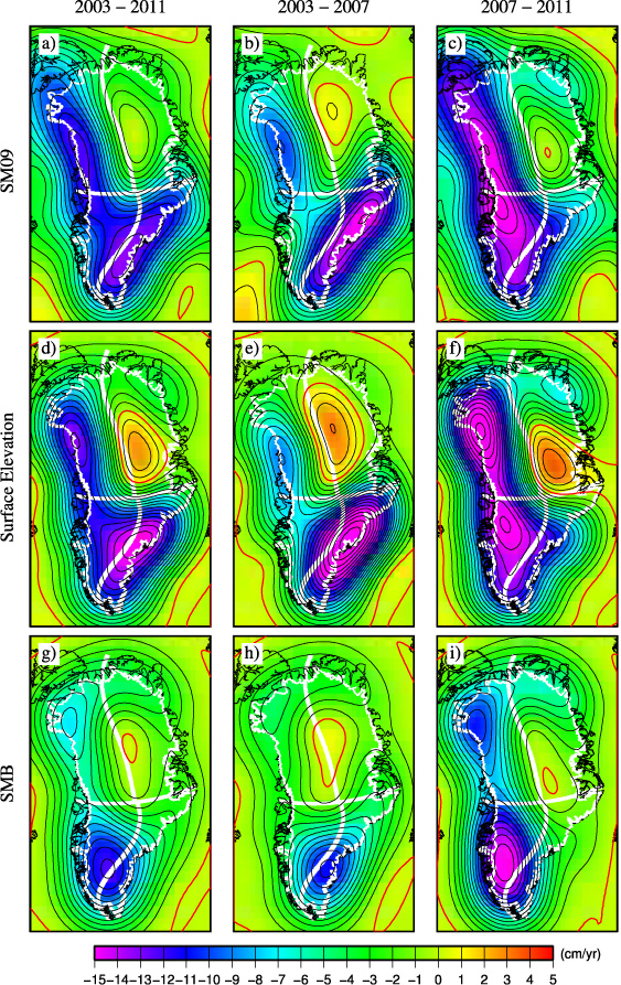
Figure 2. Greenland ice mass and elevation changes. (a)–(c) GRACE ice mass changes corrected using SM09-GIA in cm yr−1 of water; (d)–(f) altimetry measurements of ice volume change corrected using SM09-GIA in cm yr−1 of surface elevation; (g)–(i) RACMO SMB changes in cm yr−1 of water for the time periods ((a), (d), (g)) September 2003–August 2011, ((b), (e), (h)) September 2003–September 2007, ((c), (f), (i)) September 2007–August 2011. Red line denotes the contour at 0 cm yr−1. White lines define the four regions, NW, NE, SW and SE.
Download figure:
Standard image High-resolution image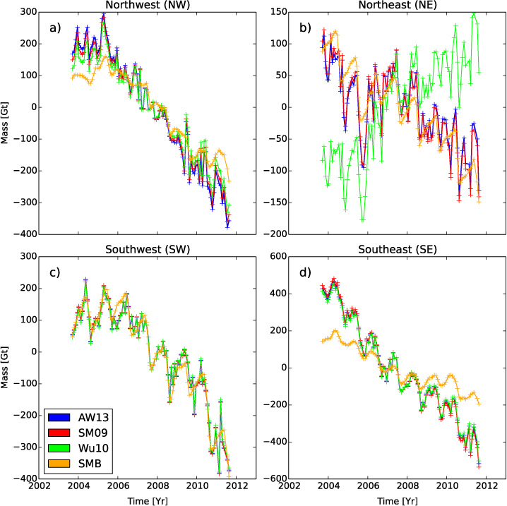
Figure 3. Ice mass changes for the time period September 2003–August 2011 in Gigatons (1 Gt = 1012 kg) for the four regions (a) NW, (b) NE, (c) SW and (d) SE Greenland shown in figure 1. GRACE ice mass estimates calculated using AW13-GIA (blue), SM09-GIA (red), Wu10-GIA (green), and RACMO SMB (orange) are shown.
Download figure:
Standard image High-resolution image
Acknowledgments
We thank the editor and two anonymous reviewers for their advice. This work was performed at the University of California Irvine, the Jet Propulsion Laboratory, California Institute of Technology, and was supported by grants from NASA's Cryospheric Science Program, Solid Earth and Natural Hazards Program, Terrestrial Hydrology Program, IDS Program, and MEaSUREs Program. Maps have been drawn using Generic Mapping Tools (GMT) (Wessel and Smith 1998). Computations were performed with Python for Scientific Computing (Oliphant 2007). Time series plots were drawn using the matplotlib graphics environment (Hunter 2007).