
Abstract
Glacier mass changes are a valuable indicator of climate variability and monsoon oscillation on the underexplored Tibetan Plateau. In this study data from the Ice Cloud and Elevation Satellite (ICESat) is employed to estimate elevation and mass changes of glaciers on the Tibetan Plateau between 2003 and 2009. In order to get a representative sample size of ICESat measurements, glaciers on the Tibetan Plateau were grouped into eight climatically homogeneous sub-regions. Most negative mass budgets of − 0.77 ± 0.35 m w.e. a−1 were found for the Qilian Mountains and eastern Kunlun Mountains while a mass gain of + 0.37 ± 0.25 m w.e. a−1 was found in the westerly-dominated north-central part of the Tibetan Plateau. A total annual mass budget of − 15.6 ± 10.1 Gt a−1 was estimated for the eight sub-regions sufficiently covered by ICESat data which represents ∼80% of the glacier area on the Tibetan Plateau. 13.9 ± 8.9 Gt a−1 (or 0.04 ± 0.02 mm a−1 sea-level equivalent) of the total mass budget contributed 'directly' to the global sea-level rise while 1.7 ± 1.9 Gt a−1 drained into endorheic basins on the plateau.
Export citation and abstract BibTeX RIS

Content from this work may be used under the terms of the Creative Commons Attribution 3.0 licence. Any further distribution of this work must maintain attribution to the author(s) and the title of the work, journal citation and DOI.
1. Introduction
The Tibetan Plateau (TP) with an average altitude of more than 4000 m above sea-level is characterized by the presence of many glaciers and ice caps. The climate of the TP is mainly governed by the westerlies, as well as the south Asian and the south-east Asian monsoons. Since the magnitude of these climatic influences varies, different types of glaciers are present from maritime or temperate-type glaciers in the south-east to continental or polar-type glaciers in the north-west (Shih et al 1980, Huang 1990). However, direct measurements of climatic parameters are sparse, especially in the western part of the TP and the circulation pattern of the monsoon system is still not fully understood. The variability of glaciers is a valuable indicator for climate variability in remote regions (e.g. Yao et al 2012). Furthermore a quantification of melt water recharge of Tibetan glaciers would help to understand the role of different climate components (temperature, precipitation and evaporation) in the lake-level oscillation of numerous lakes on the TP (Zhang et al 2011, Kropáček et al 2012, Phan et al 2012, Zhang et al 2013). Lake-level changes are also of direct impact to the local population as increasing levels are flooding pastures (Yao et al 2007).
In the last decade several studies used remote sensing techniques to account for areal changes of glaciers in this large and remote region (e.g. Ding et al 2006, Liu et al 2006, Ye et al 2006, Bolch et al 2010). However, glacier area changes provide only an indirect signal while the glacier mass budget shows the immediate reaction to climate variability (Oerlemans 2001). Laser altimetry data acquired by the Geoscience Laser Altimeter System (GLAS) carried on-board the Ice Cloud and Elevation Satellite (ICESat) were proven to be an accurate data source for the regional estimation of glacier elevation changes (Kääb et al 2012, Bolch et al 2013, Gardner et al 2013). Kääb et al (2012) estimated trends in glacier elevation changes for the Himalaya and Hindu Kush region leaving the TP unobserved. A recent study estimated global glacier mass changes using glaciological mass balance measurements, data from the Gravity Recovery And Climate Experiment (GRACE) and ICESat data, including High Mountain Asia (Gardner et al 2013). In this study we focus in detail on trends in glacier elevation and mass changes within eight sub-regions on the TP (figure 1) for the last decade and discuss our results in comparison to existing, but sparse, in situ measurements and recent remote sensing studies (e.g. Yao et al 2012, Gardner et al 2013, Neckel et al 2013). The investigated region contains a total ice cover of ∼32 400 km2 according to the first Chinese Glacier Inventory (CGI) (Li 2003, Shi et al 2009) which accounts for ∼80% of the Tibetan ice cover.
2. Data and method
ICESat GLAS data and the digital elevation model (DEM) acquired by the Shuttle Radar Topography Mission (SRTM) in February 2000 (Rabus et al 2003, Farr et al 2007) were employed to calculate volume changes of Tibetan glaciers. ICESat was launched in January 2003 hosting three laser sensors within the GLAS. The laser channels for surface altimetry operated at a wavelength of 1064 nm with footprints spaced at about 172 m along track and a diameter on the surface of about 70 m (Zwally et al 2002, Brenner et al 2003). The ICESat mission was conducted during 18 laser periods, each lasting between 12 and 55 days. As ICESat's precision spacecraft pointing control was not used in mid-latitudes between 59°S and 59°N individual repeated tracks do not match exactly but can be separated across track by up to 3000 m in our study area. Due to this fact and because of the rugged topography of the TP, cross-over and along-track processings of ICESat data (e.g. Brenner et al 2007, Slobbe et al 2008, Moholdt et al 2010) cannot be applied here. However, two recent studies proved the suitability of ICESat data in deriving elevation changes of mountain glaciers (Kääb et al 2012, Gardner et al 2013). Similar to Rinne et al (2011), Kääb et al (2012) and Gardner et al (2013) we used an independent DEM as a reference surface on which we compared ICESat elevation measurements. In this study we used version 3 of the SRTM C-band DEM (90 m grid spacing, hereinafter SRTM-C DEM).
Glaciers on the TP are small compared to the large polar ice sheets and ice caps and ICESat measurements over Tibetan glaciers are sparse. However, a sufficient number of ICESat measurements acquired in one track is needed in order to perform a statistical sound analysis. Therefore glaciers were grouped into eight compact sub-regions where we assume climatologically homogeneous conditions (figure 1). In order to test if the selected sub-regions are sufficiently covered by ICESat measurements we compared the area elevation distribution of the ICESat measurements with the glacier hypsometry in all sub-regions (figure S1(a), avaialable at stacks.iop.org/ERL/9/014009/mmedia). For most sub-regions the deviation is within ± 15% with the highest deviation of + 20% in sub-region F. Additionally, we conducted a bootstrapping analysis in which we iteratively included a random selection of ICESat footprints (figure S2, avaialable at stacks.iop.org/ERL/9/014009/mmedia). Both analyses confirm that the eight sub-regions are covered relatively well by the ICESat dataset. The eight sub-regions contain a total ice cover of ∼32 400 km2 which accounts for ∼ 80% of the glacier area on the TP. As the CGI tends to be spatially inaccurate, ICESat measurements on glaciers were manually selected based on the most recent cloud free Landsat scenes (Thematic Mapper, Level 1, acquisition between 2003 and 2011) obtained from the web archive of the USGS.
We used bilinear interpolation to extract the SRTM-C surface elevation, at the exact location of each ICESat measurement. ICESat measurements were excluded from the analysis if the difference between ICESat and SRTM-C elevation exceeded 150 m, which is attributed to cloud cover or atmospheric noise during the time of data acquisition. The elevation difference ΔH between each ICESat footprint and the SRTM-C DEM was calculated by

where HICESat and HSRTM are the elevation measurements of both datasets. As on the TP most glaciers receive very low precipitation rates predominantly occurring in the summer (Ageta and Fujita 1996, Böhner 2006, Maussion et al 2013), multi-seasonal linear trends were fitted through all ΔH values. In order to make our results comparable to other studies we calculated mass balance estimates in water equivalent (w.e.), using the CGI for information on glacier area (Li 2003, Shi et al 2009). For volume to mass conversion we used an average ice density of 850 ± 60 kg m−3 (Huss 2013). Mass balance estimates were calculated for all glaciers covered by ICESat. An area weighted upscaling was performed for each sub-region using the CGI for information on glacier area. For the calculation of the percentage of glacier area draining into endorheic basins we employed the HydroSHEDS dataset (Lehner et al 2006). Following Kääb et al (2012) mass balances were also calculated from ΔH trends, solely based on autumn acquisitions (table S2 and figure S8 available at stacks.iop.org/ERL/9/014009/mmedia).
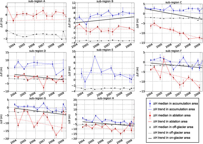
Considering glacier flow, mass balance estimates were calculated for ΔH trends integrated over the entire glacier area. However, in order to look at differences in glacier thinning with respect to altitude, to detect unusual behavior such as glacier surging and to discuss the influence of surface elevation gain due to possible snow accumulation we also calculated ΔH trends separately for the accumulation and ablation areas in each sub-region (figure 2). The equilibrium line altitude (ELA) values used for the separation into accumulation and ablation areas are shown in table S1 available at stacks.iop.org/ERL/9/014009/mmedia.
Table 1. Regional trends of glacier elevation changes are shown next to the area weighted mass balance, total glacier area in each sub-region and the percentage of the glacier area in each sub-region draining into endorheic basins. Geographic location of sub-regions is shown in figure 1 and trend lines are shown in figure 2. Statistical significant trends are illustrated as bold numbers.
| Sub-region | ΔH trend accumulation area (m a−1) | ΔH trend ablation area (m a−1) | ΔH trend on-glacier area (m a−1) | ΔH trend off-glacier area (m a−1) | Mass balance (m w.e. a−1) | Total glacier area (km2) | Drainage into endorheic basins (%) |
|---|---|---|---|---|---|---|---|
| A | — | + 0.04 ± 0.29 | + 0.04 ± 0.29a | − 0.11 ± 0.08 | + 0.03 ± 0.25a | 6 483 | 43 |
| B | + 0.50 ± 0.30 | − 0.05 ± 0.26 | + 0.44 ± 0.26 | + 0.02 ± 0.02 | + 0.37 ± 0.25 | 464 | 100 |
| C | − 0.45 ± 0.31 | − 1.40 ± 0.51 | − 0.90 ± 0.28 | − 0.09 ± 0.05 | − 0.77 ± 0.35 | 1 491 | 100 |
| D | + 0.55 ± 0.33 | − 0.68 ± 0.35 | − 0.68 ± 0.29 | − 0.04 ± 0.02 | − 0.58 ± 0.31 | 1 859 | 30 |
| E | − 0.23 ± 0.33 | — | − 0.23 ± 0.33b | + 0.01 ± 0.02 | − 0.20 ± 0.29b | 1 056 | 38 |
| F | − 0.31 ± 0.28 | − 1.30 ± 0.47 | − 0.44 ± 0.26 | + 0.02 ± 0.02 | − 0.37 ± 0.25 | 2 371 | 42 |
| G | − 0.46 ± 0.31 | − 1.15 ± 0.44 | − 0.78 ± 0.27 | + 0.03 ± 0.04 | − 0.66 ± 0.32 | 6 632 | 2 |
| H | − 0.71 ± 0.38 | − 0.85 ± 0.41 | − 0.81 ± 0.32 | + 0.15 ± 0.07 | − 0.69 ± 0.36 | 12 017 | 0 |
aData only available in ablation area. bData only available in accumulation area.
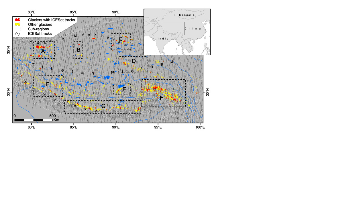
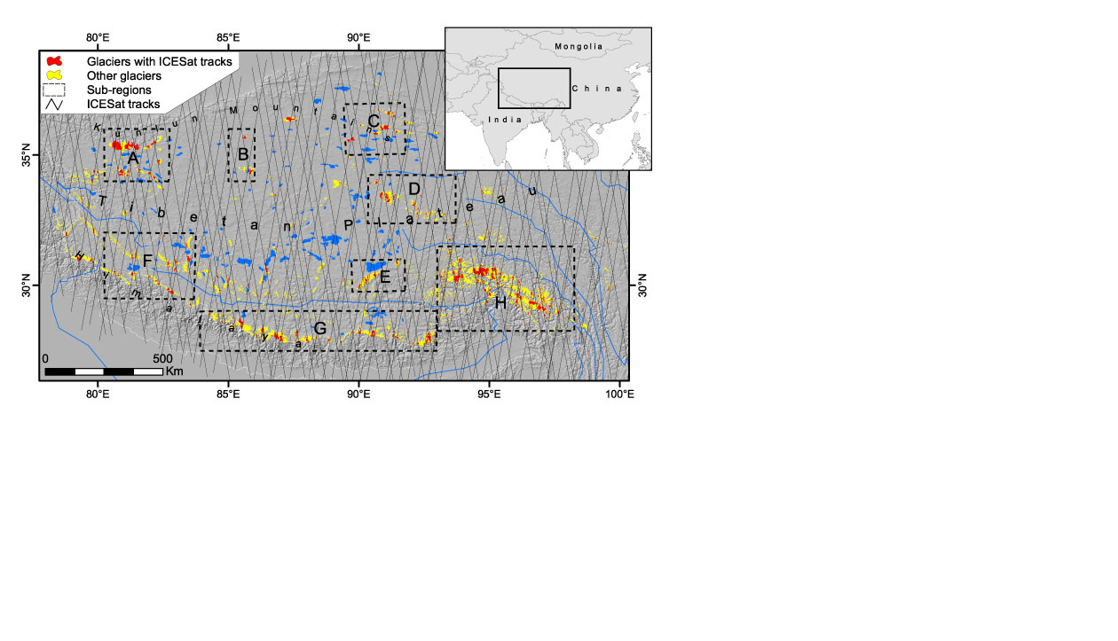
Figure 1. Overview of the study area including ICESat data coverage. Glacier outlines are based on the Chinese Glacier Inventory (CGI) (Li 2003, Shi et al 2009). Sub-regions are marked as black boxes and are sorted by alphabetical order with A = western Kunlun Mountains, B = Zangser Kangri and Songzhi Peak, C = Qilian Mountains and eastern Kunlun Mountains, D = Tanggula Mountains and Dongkemadi Ice Cap, E = western Nyainqentanglha range, F = Gangdise Mountains, G = central and eastern Tibetan Himalaya, H = eastern Nyainqentanglha range and Hengduan Mountains.
Download figure:
Standard image High-resolution image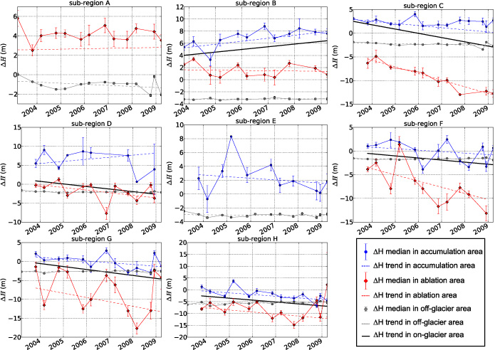
Figure 2. Estimated trends for selected geographic sub-regions as shown in figure 1. Trends were fitted through all ΔH values in on- and off-glacier areas. For on-glacier areas trends are shown separately for the accumulation and ablation areas as well as for the whole glacier area. For clarity reasons only the ΔH median of each laser period is shown. Year dates correspond to 1 January of each year.
Download figure:
Standard image High-resolution image
Figure 3. Mass balance estimates in m w.e. a−1 derived from ICESat measurements in comparison to in situ mass balance measurements of single glaciers (2006–2010, Yao et al 2012).
Download figure:
Standard image High-resolution image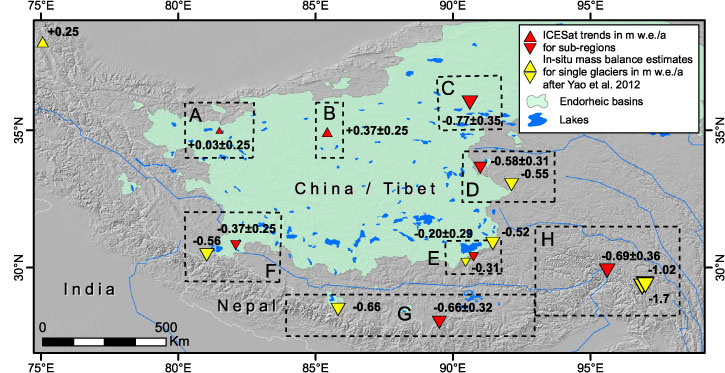
3. Results
Our results reveal a heterogeneous wastage of glaciers and ice caps across the TP (figure 2, table 1). It should be noted, that ΔH trends were fitted through all ΔH values, however for a better visual representation only the ΔH median of each laser period is shown in figure 2. Due to this fact, small offsets may occur between the ΔH medians and the trend lines (e.g. in sub-region A). The separate calculation of ΔH trends in the accumulation and ablation area revealed an offset of several meters between both trends in each sub-region (figure 2) which can be attributed to the different penetration of the SRTM C-band into snow, firn and ice (Rignot et al 2001, Gardelle et al 2012).
We determined on average a decrease of glacier surface elevations between 2003 and 2009 but also found positive trends for two sub-regions. The highest specific mass loss was found for the Qilian Mountains and eastern Kunlun Mountains (− 0.77 ± 0.35 m w.e. a−1) located in the north-eastern part of the TP, the eastern Nyainqentanglha range and Hengduan Mountains (− 0.69 ± 0.36 m w.e. a−1) and the central and eastern Tibetan Himalaya (− 0.66 ± 0.32 m w.e. a−1), regions which are predominantly monsoon-influenced. In contrast, the continental westerly-influenced north-western (western Kunlun Mountains) and north-central mountains (Zangser Kangri and Songzhi Peak) showed evidence for balanced mass budgets or a slight mass gain. For the latter peaks which are covered by ice caps, we detected glacier thinning at lower elevations while a simultaneous glacier thickening was observed at higher elevations (figure 2, sub-region B). The same altitude depended pattern is found for the Tanggula Mountains and Dongkemadi Ice Cap (figure 2, sub-region D), except that the overall mass balance is negative in this sub-region (− 0.58 ± 0.31 m w.e. a−1). The western Kunlun Mountains (sub-region A) are characterized by a heterogeneous behavior of glacier elevation changes. Here we found significant surface lowering in the accumulation areas of some glaciers with a simultaneous elevation increase at ICESat footprints in ablation areas, indicating the occurrence of glacier surges in this sub-region. The highest mass loss and contribution to sea-level rise is comprised from the strongly glacerized eastern Nyainqentanglha range and Hengduan Mountains with − 8.3 ± 4.3 Gt a−1 (or 0.02 ± 0.01 mm a−1 sea-level equivalent, sub-region H). In sum, we estimated a total annual mass budget of − 15.6 ± 10.1 Gt a−1 for the eight sub-regions, of which 1.7 ± 1.9 Gt a−1 were not leaving the TP as stream flow but drained into endorheic lakes on the plateau. Glaciers draining into the endorheic Tarim Basin in the north of the TP showed on average balanced mass budgets.
4. Discussion
In this study two almost global datasets, the ICESat GLA 14 product and the SRTM-C DEM were used to conduct a regional study of trends in glacier surface elevation changes. The main problem when utilizing ICESat data to estimate elevation changes of glaciers in mid-latitudes is the large distance between ICESat tracks and the corresponding limited data coverage of mountain glaciers. However, recent studies have proven that ICESat is an accurate data source if the available data sample is statistically suitable for a region, i.e. if the investigated region and its ice covered area is large enough (Kääb et al 2012, Bolch et al 2013, Gardner et al 2013). In our approach, we assume no prominent snow accumulation period in high elevations on the TP and fitted trends through multi-seasonal ICESat acquisitions. This way, the statistical significance increased due to a higher number of measurements in the data-sparse sub-regions. On the TP a multi-seasonal data fit can be justified for several reasons. (1) The north-western part of the plateau receives very low precipitation rates in winter, although winter precipitation is predominant in this region (Böhner 2006). (2) In the south-eastern part accumulation and ablation at higher elevations is related to monsoon precipitation in summer (Ageta and Fujita 1996, Kang et al 2009). (3) A recent study of Maussion et al (2013) showed that the majority of glaciers on the central TP are accumulating mass in summer. (4) We also conducted our analysis solely based on autumn acquisitions (figure S8 and table S2, available at stacks.iop.org/ERL/9/014009/mmedia). The resulting trends are similar as for the multi-seasonal data and agree within their error bars. The mean and maximum difference between the multi-seasonal ΔH trends and the autumn ΔH trends were estimated at 0.06 m a−1 and 0.33 m a−1 respectively. However, the sparser sampling distribution of the autumn laser periods led to statistical insignificant ΔH trends in some of the sub-regions.
Our study tends to agree with other studies which show similar regional patterns of glacier changes in the Himalaya (Bolch et al 2012, Kääb et al 2012, Gardelle et al 2013) and on the TP (figure 3) (Yao et al 2012, Gardner et al 2013). However, we show some more details on the spatial variability within Tibet and consider also the drainage into endorheic basins separately.
The bigger picture shows an overall negative trend in glacier mass budgets with the highest specific mass loss in the monsoon-influenced north-eastern and south-eastern margins and balanced mass budgets in the more westerly-influenced north-western regions. A direct comparison between the studies is difficult as the studied sub-regions are not identical and the time span of observations is also partly different.
For the western Kunlun Mountains (sub-region A), we estimated slightly positive trends in glacier elevation changes. However, we found strong data noise of up to ± 80 m for ΔH in the accumulation area so that no meaningful trend could be derived here. Although our estimate of + 0.04 ± 0.29 m a−1 in the ablation area is not statistically significant a balanced glacier regime can be assumed for the western Kunlun Mountains which is in agreement with Gardner et al (2013). It should be noted that large variations in glacier area changes with several advancing glaciers are reported in this region (Shangguan et al 2007, Scherler et al 2011, Yao et al 2012). Also the results of Maussion et al (2013) suggest different accumulation regimes for the north and south facing slopes of the western Kunlun Mountains. Our study seems to confirm that the western Kunlun Mountains show a similar anomaly than the neighboring Pamir and also the Karakoram Mountains (Gardelle et al 2013). However, this possible western Kunlun anomaly needs further investigation as our study revealed that the ICESat estimate stretches its limits in sub-regions with heterogeneous behavior of glaciers. It is therefore recommended to calculate ΔH trends separately for the accumulation and ablation areas.
Possible positive mass budgets were also found for the large ice fields of Zangser Kangri and Songzhi Peak (sub-region B). Here we found a positive trend in the accumulation area, while glacier thinning was observed in lower regions suggesting strong firn and snow accumulation. We therefore tested a lower density of 600 kg m−3 for the conversion from volume to mass which revealed a smaller mass gain of + 0.26 ± 0.18 m w.e. a−1. This value seems more appropriate than the proposed estimate of + 0.37 ± 0.25 m w.e. a−1 (table 1) but is also covered by our error estimate.
For the Tanggula Mountains and Dongkemadi Ice Cap (sub-region D) the overall trend follows the trend of the ablation area due to sparse data sampling in the accumulation area. However, strong mass loss in ablation regions led to an overall significant negative mass budget for this sub-region. Such a behavior is also common for ice caps in arctic regions (Gardner et al 2011, Bolch et al 2013) while on the central TP (e.g. in sub-region B) the mass loss in the ablation area is probably compensated by strong accumulation (Neckel et al 2013).
Our results for the central and eastern Tibetan Himalaya are in agreement with Gardner et al (2013) (sub-region G, this study: − 0.78 ± 0.27 m a−1, Gardner et al (2013): − 0.89 ± 0.18 m a−1) but are clearly more negative than the values from Kääb et al (2012). The difference is difficult to investigate as the sample regions do not match and therefore different glaciers were sampled. Similar to the Himalayan region, the ICESat derived mass budgets for the eastern Nyainqentanglha range and the Hengduan Mountains (sub-region H) are more negative than the results based on DEM differencing between 1999 and 2010 (Gardelle et al 2013). The authors of the latter study state in their paper that mass losses measured with ICESat tend to be slightly larger than their estimates. In addition, different glaciers were measured over a slightly different time span in both studies, making a direct comparison difficult.
Our results seem to be in contradiction to the findings of Jacob et al (2012) which showed an increase in mass from GRACE measurements between 2003 and 2010 on the TP. However, a recent study by Zhang et al (2013) attributed this increase in mass predominately to an increase in lake level/mass rather than to an increase in glacier mass. This observation is in agreement with our study as most of the eight sub-regions showed a negative mass balance for the studied time period. However, the estimated negative mass budgets could not be detected by GRACE as many glaciers on the TP drain into endorheic lakes. This amount is estimated at 1.7 ± 1.9 Gt a−1 in this study. It should therefore be noted that only 13.9 ± 8.9 Gt a−1 (or 0.04 ± 0.02 mm a−1 sea-level equivalent) of our total annual mass budget estimate can directly contribute to the global sea-level rise, while the majority of the remaining mass loss can likely be linked to the observed rise of the lake levels (Zhang et al 2011, Kropáček et al 2012, Phan et al 2012). Similar to the fact that the rising sea-level threatens coastal areas on the globe, the rising lake levels pose problems to the local population as pastures are often situated close to the lakes and will be flooded (e.g. Yao et al 2007).
5. Conclusions
This study presents glacier surface elevation changes and mass budget estimations for almost the entire TP for the period 2003 – 2009 including central TP where no previous mass balance estimates exist. The fitting of multi-seasonal ICESat elevation differences in combination with density assumptions enabled us to derive meaningful estimates of glacier mass changes for eight detailed sub-regions on the TP. A total annual mass budget of − 15.6 ± 10.1 Gt a−1 was estimated for the eight sub-regions which includes ∼80% of the glacier area on the TP. Of the estimated total mass budget 13.9 ± 8.9 Gt a−1 (or 0.04 ± 0.02 mm a−1 sea-level equivalent) contributed directly to the global sea-level rise while 1.7 ± 1.9 Gt a−1 drained into endorheic basins, i.e. were not leaving the TP as stream flow. Glaciers in the north-central part of the TP were probably gaining mass while glaciers in the south-eastern part were significantly loosing mass between 2003 and 2009. These trends were found to be in agreement with the few existing in situ mass balance measurements and several recent remote sensing studies. Hence, this study confirms that ICESat data in combination with a detailed DEM provides a valuable source of information about elevation changes of mountain glaciers on a regional scale.
Acknowledgments
This work was supported by the German Federal Ministry of Education and Research (BMBF) Programme Central Asia—Monsoon Dynamics and Geo-Ecosystems (CAME) within the WET project (Variability and Trends in Water Balance Components of Benchmark Drainage Basins on the Tibetan Plateau) under the code 03G0804D and by the German Research Foundation (DFG) Priority Programme 1372, Tibetan Plateau: Formation—Climate—Ecosystems within the DynRG-TiP (Dynamic Response of Glaciers on the Tibetan Plateau to Climate Change) project under the code BU 949/20-3. T Bolch acknowledges the funding through DFG (BO 3199/2-1) and the European Space Agency (ESA) project Glaciers_cci (400010177810I-AM). We are thankful for the cooperation with the Institute for Tibetan Plateau Research (ITP), Beijing. We acknowledge NSIDC for hosting the ICESat data and the CGI dataset. SRTM-C data and Landsat imagery were obtained from the USGS. The valuable comments of two anonymous referees and of the scientific editor significantly improved the letter.