
Abstract
Subgrid-scale variability is one of the main reasons why parameterizations are needed in large-scale models. Although some parameterizations started to address the issue of subgrid variability by introducing a subgrid probability distribution function for relevant quantities, the spatial structure has been typically ignored and thus the subgrid-scale interactions cannot be accounted for physically. Here we present a new statistical-physics-like approach whereby the spatial autocorrelation function can be used to physically capture the net effects of subgrid cloud interaction with radiation. The new approach is able to faithfully reproduce the Monte Carlo 3D simulation results with several orders less computational cost, allowing for more realistic representation of cloud radiation interactions in large-scale models.
Export citation and abstract BibTeX RIS

Content from this work may be used under the terms of the Creative Commons Attribution 3.0 licence. Any further distribution of this work must maintain attribution to the author(s) and the title of the work, journal citation and DOI.
1. Introduction
Parameterizations in a global climate model (GCM) are designed to describe the 'collective effects' of processes that occur at scales smaller than GCM grid sizes (Randall et al 2003). Parameterizations of many processes such as radiation transfer and autoconversion employ the assumption of independent column approximation (ICA), i.e., there is no interaction between subcolumns and the grid-average effects depend only on the probability distribution function (PDF) of relevant variables (Pincus et al 2003). ICA approaches use one-point statistical information (e.g., PDF), called subgrid variability in this letter and structural information (e.g., spatial organization and arrangement) that can be characterized by multi-point statistics is generally ignored. However, coherent structures have been found at scales ranging from droplet clusters to organized cloud, and have complex interactions with radiation, dynamical processes, and mesoscale environment systems (Kostinski and Shaw 2001, Marshak et al 2005, Feingold et al 2010). Failure to include subgrid cloud and convection structures can lead to inadequate simulations of large-scale features (Lin et al 2011). It has been found that ignoring cloud spatial organization tends to underestimate or overestimate the domain-average radiation fluxes dependent on many factors, e.g., solar angle and cloud geometry (Zuidema and Evans 1998, Barker et al 1999, Scheirer and Macke 2003, Davis and Mineev-Weinstein 2011, Hogan and Shonk 2013).
Given the detailed cloud field, the radiation field can be found by numerically solving the 3D transport equation (Evans 1998). In many applications, the knowledge of 3D cloud field is unavailable or expensive to obtain. It is often difficult to draw any theoretical conclusion based on the 3D approach: there could be numerous configurations of 3D cloud field that will give statistically similar radiation characteristics (Anisimov and Fukshansky 1992). Besides these, numerically solving the 3D problem is too expensive to use in practical applications. In climate models, it is a standard practice to employ the ICA assumption, i.e., divide the domain into two (clear and cloudy) or more subcolumns (Pincus et al 2003, Shonk and Hogan 2008) and independently calculate the radiation flux within each subcolumn.
Previous efforts on parameterization of 3D cloud-radiation interaction in large-scale models have focused on binary medium or oversimplified closure assumptions (Anisimov and Fukshansky 1992, Vainikko 1973, Titov 1990, Pomraning 1996, Tompkins and Di Giuseppe 2007, Stephens 1988, Kassianov and Veron 2011, Hogan and Shonk 2013). Here we present a new statistical physics-like simulation approach that makes a direct connection between the statistical characterization of cloud structure and the statistical moments of the radiation field by properly averaging the 3D equation. The unknowns of the resultant statistical radiative transport (SRT) equations are actually the statistical moments of the radiation field, and the model inputs are some statistical moments of the 3D medium structure. In this letter, we show that a spatial correlation function can serve as the key to statistically describing cloud–radiation interactions.
2. Basic theory and method
To examine what structural information is needed for the transport problem, let us consider radiation transfer in a cloudy atmosphere vertically confined within [0, 1] where the top is at z = 0. The monochromatic radiance at r = (x, y, z) in direction  is denoted by I(r, Ω), where
  is the cosine of the zenith angle and
  is the azimuth angle. The solar radiance field satisfies the 3D radiative transfer equation of integral form (Chandrasekar 1950):
where  , I(rb
, Ω) is the incoming solar radiance at the upper boundary for downward directions (μ < 0) and is the surface reflection for upward directions (μ > 0); σ(r) and ω0(r) are respectively the cloud extinction coefficient and single scattering albedo; and p(r, Ω', Ω) is the scattering phase function. The second term on the left-hand side is the path extinction and the first term on the right-hand side is the source due to scattering. Note that the extinction coefficient is normalized with regard to the depth of the atmosphere layer and its integral over [0, 1] corresponds to the optical depth of the cloudy atmosphere. The interval of integral is given by E = [0, z] for downward directions and E = [z, 1] for upward directions. Here we trintroduce the ergodic hypothesis, which implies that the ansport processes should possess certain translational invariance in spatial coordinate and thus lead to the equality of ensemble and spatial averages (Titov 1990, Rybicki 1965). It is feasible to assume that the deterministic transfer equation is valid for each member of the ensemble system. Therefore, statistics is introduced only to account for the lack of knowledge about the detailed structure of the cloud, not about the equations governing the transport processes.
, I(rb
, Ω) is the incoming solar radiance at the upper boundary for downward directions (μ < 0) and is the surface reflection for upward directions (μ > 0); σ(r) and ω0(r) are respectively the cloud extinction coefficient and single scattering albedo; and p(r, Ω', Ω) is the scattering phase function. The second term on the left-hand side is the path extinction and the first term on the right-hand side is the source due to scattering. Note that the extinction coefficient is normalized with regard to the depth of the atmosphere layer and its integral over [0, 1] corresponds to the optical depth of the cloudy atmosphere. The interval of integral is given by E = [0, z] for downward directions and E = [z, 1] for upward directions. Here we trintroduce the ergodic hypothesis, which implies that the ansport processes should possess certain translational invariance in spatial coordinate and thus lead to the equality of ensemble and spatial averages (Titov 1990, Rybicki 1965). It is feasible to assume that the deterministic transfer equation is valid for each member of the ensemble system. Therefore, statistics is introduced only to account for the lack of knowledge about the detailed structure of the cloud, not about the equations governing the transport processes.
We further assume that the scattering phase function p and single scattering albedo ω0 depend only on height z. Let <···> denote the horizontal or ensemble average, the vertical profile of horizontally-averaged radiance can be obtained after applying the notations

This averaging process is conceptually similar to the Reynolds averaging widely used in fluid dynamics (Reynolds 1895). The domain-average radiance  is now explicitly presented in equation (2) but the equation is not closed since a new variable
  still needs to be determined. The variable
  is the mean product of radiance and extinction coefficient and, with the assumption of horizontally-invariant single scatter albedo, radiation absorption A at any level can be readily found by:
![$A(z)=\left[ 1-{{\omega }_{0}}(z) \right]\int 4\pi \bar{U}(z,{\boldsymbol{ \Omega }} ){\rm d}{\boldsymbol{ \Omega }} $](https://content.cld.iop.org/journals/1748-9326/9/12/124022/revision1/erl506246ieqn8.gif) . Multiplying equation (1) with σ(r) and performing the horizontal average again, we obtain an equation for
. Multiplying equation (1) with σ(r) and performing the horizontal average again, we obtain an equation for  :
:
To solve this equation, we can either truncate the higher order terms at certain point, or introduce independent hypotheses of closure to determine the higher order terms in terms of the lower order ones. Here the second approach is used. We modified the standard Intercomparison of 3D Radiation Codes (I3RC) community Monte Carlo model (Cahalan et al 2005, Pincus and Evans 2010) to compute and record 3D radiance field. Based on the analysis of Monte Carlo simulations with a variety of cloud cases (the supplementary material, available at stacks.iop.org/ERL/9/124022/mmedia provides some details on how the closure is derived), the higher order term  can be approximated in two steps:

 is the spatial covariance function of cloud extinction coefficients at levels z and z' along the direction Ω and, with an appropriate normalization, it becomes the spatial autocorrelation function. For the rest of this letter, the terms covariance and autocorrelation are interchangeable. The correlation function provides a measure of the spatial structure of cloud extinction coefficient.
![${\Delta }x\in [0,\infty ],{\Delta }y\in [0,\infty ]\}$](https://content.cld.iop.org/journals/1748-9326/9/12/124022/revision1/erl506246ieqn13.gif) , i.e., the minimum autocorrelation at level z'. The coefficients f2 and f3 depend only on the horizontal average (
, i.e., the minimum autocorrelation at level z'. The coefficients f2 and f3 depend only on the horizontal average ( ) and variance (V) of cloud extinction coefficient in the corresponding layer:
  and
and  . It can be verified that, for binary media, equations (4a) and (4b) will converge to the closure scheme of Titov (1990) that was specifically designed for binary media. To accurately calculate the direct (unscattered) radiation, knowledge about the PDF of extinction coefficient may also be needed.
Given the closure scheme of equation (4), the weighted mean radiation field  can be determined by analytically or numerically solving the 1D Volterra integral equation (3) and then the mean radiation field
  can be readily obtained through equation (2).
It can be seen from equations (3) and (4) that the term  is the key to describing the interaction between the 3D radiation and cloud fields; the function
  serves as a direct linkage between the mean radiation field and 3D cloud structure and encapsulates information of the 3D cloud structure across various spatial scales. Figure 1 shows an example of spatial correlation function for a 3D cloud field simulated by a large eddy simulation model (Pincus and Evans 2010). When the separation distance is zero, the cloud field at r' = r perfectly correlates with itself, i.e.,
 . The correlation function approaches the asymptote
  , i.e., statistically independent, once the separation distance becomes large enough. The decorrelation length is related to mean cloud size in the x-dimension in this example. It should be noted that the correlation function can also be smaller than
  if the properties are negatively correlated.
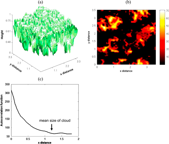
Figure 1. Spatial autocorrelation function of a stratocumulus cloud. (a) 3D rendering of the isosurface at extinction coefficient value of 20; (b) a horizontal cross section of the 3D cloud extinction coefficient field at z = 0.6; and (c) the spatial autocorrelation function of this cross section along the x direction.
Download figure:
Standard image High-resolution image3. Numerical results
To evaluate the new approach, we perform a suite of numerical simulations using a discrete ordinate method for angular discretization (Bass et al 1986). The angular discretization uses an equal-area Carlson quadrature scheme and therefore both the latitudinal and longitudinal variations are represented by the discrete ordinates. The spatial (vertical) discretization is chosen to make the mean optical depth of each layer not exceeding 1. Equation (3) is now converted to a system of linear equations with the vertical and angular discretizations. To use efficient solvers like DISORT (Stamnes et al 1988), further simplifications of equation (3) will be required. Since the purpose of this letter is to demonstrate the viability of the SRT approach, further simplification and numerical optimization will be the topic of a future research. A successive order approximation is used to simulate multiple scattering where the lower order scattering serves as the source for the higher order calculation (Shabanov et al 2000). For the zero-order radiation calculation, the source function is set to be unit which corresponds to a collimate incident beam without any diffuse component. The first-order scattering is then determined with the source function based on the zero-order solution. This process is repeated until the solution converges with a prescribed criteria. For the medium with a very large optical thickness, a large number of vertical layers may be needed and the successive order approximation method can be tedious. For all simulations performed in this research, we assume perfect knowledge about the cloud spatial correlation functions so that the accuracy of the second order closure scheme (equation (4)) can be evaluated against the full 3D Monte Carlo results (Barker et al 1999).
To examine the impacts of ignoring cloud structure, called 3D effects here, we also compare the SRT results with two widely-used approximation methods: Plane-parallel approximation (PPA) and ICA (Barker et al 1999, Oreopoulos and Barker 1999, Barker and Davis 2005). The PPA approach assumes plane parallel geometry with each layer taking horizontal mean optical properties and ignores the horizontal fluctuations. The ICA approach assumes no net horizontal transport of particles or photons between columns so that the mean radiation characteristics can be obtained by solving a1D deterministic transport equation for each column and averaging the resultant solutions.
The first group of simulations are based on an idealized checkerboard-like medium as shown in figure 2(a); this case is notoriously challenging for 1D transport models since its exaggeration of 3D transport effects (Wiscombe 2005). The optical thickness of the black and white cells is 18 and 0. The aspect ratio of each individual cell, defined as the ratio of the horizontal dimension to the vertical dimension, varies from 0.01 to 100 for different simulations. The medium is illuminated from above by collimated light at 0° or 30° zenith angles. The lateral boundary condition is assumed to be periodic and the lower boundary is ideally black. The single scattering albedo of the medium is 1. We adopt Henyey–Greenstein scattering here to represent the scattering phase function (Henyey and Greenstein 1941) and the asymmetry parameter is set to 0.85.

Figure 2. Visualization of the checkerboard medium (a), its autocorrelation functions along the x, diagonal, and z directions (b). Scene albedos are calculated with various aspect ratios using the 3D Monte Carlo, SRT, PPA, and ICA approaches for 0° (c) and 30° (d) illumination angles.
Download figure:
Standard image High-resolution imageAn aspect ratio value of 1.0 is used to obtain the two examples of spatial correlation function shown in figure 2(b). Unlike the stratocumulus cloud shown in figure 1, the spatial correlation function of the checkerboard medium is periodic and does not vanish with increasing distance. The correlation function is also capable of describing the anisotropic structures of the medium since it indicates quite different patterns along different directions.
For the 0° illumination, the scene albedo simulated by the 3D Monte Carlo method approaches 0.210 at the small aspect ratio limit and 0.292 at the large aspect ratio limit (figure 2(c)). For the 30° illumination, the scene albedo ranges from 0.310 to 0.449 for various aspect ratios (figure 2(d)). As expected, neither ICA nor PPA solutions show any dependence on the aspect ratio. The scene albedos by the PPA and ICA approaches are 0.383 and 0.296 for the 0° illumination, and 0.445 and 0.310 for the 30° illumination. The PPA albedos are always higher than others, owing to the Jensen's inequality for convex functions (Jensen 1906). The resulting albedo bias from PPA and ICA varies with aspect ratio and is up to 70% of the true albedo of the checkerboard medium.
In contrast, the SRT albedos follow closely with the 3D Monte Carlo curves over the entire range of aspect ratio, suggesting that the SRT faithfully represents the dependence of horizontal transport effects on aspect ratio. For the 0° illumination, the SRT solutions successfully reproduce the reduction of albedo that is due to radiative channeling and often found at small illumination angles, i.e., horizontal transport enhances the domain-average transmission (and suppresses reflection) relative to the ICA solutions (Davis and Marshak 2010). For a higher illumination angle, the net effect of horizontal transport is to reduce transmission (and enhance reflection) and as a result both the 3D and SRT solutions asymptote the PPA solutions at small aspect ratio limit. The horizontal transport effects are most evident when the aspect ratios are small and the discrepancy between SRT and ICA results decreases with increasing aspect ratio. When the horizontal dimension of each cell is much larger than its vertical dimension, the net effect of horizontal transport become negligible and the SRT solutions asymptote those of the ICA regardless of illumination angle. We find that whether horizontal transport enhances or suppress the scene albedo depends on many factors, including vertical and horizontal arrangement, horizontal fluctuation of optical properties of the medium, scattering phase function, and illumination angle.
The second group of simulations are for a cumulus cloud system simulated by the DARMA model (Ackerman et al 1995) shown in figure 3(a). Figure 3(b) shows the spatial autocorrelation functions of the cloud extinction at level z = 0.5 for two horizontal directions. It can be seen that the cumulus cloud appears to be statistically isotropic despite its large spatial variability. Using the more realistic cloud field may provide a better estimate of 3D effects in real world clouds. The single scattering albedo of cloud droplet is 1.0 and the scattering phase function is the same as the first case. Boundary conditions are the same as in the first case. To illustrate the dependence of horizontal transport on cloud structure, we vary the cloud aspect ratio from 0.01 to 100 to represent different levels of horizontal transport effects and keep other cloud properties fixed. Apparently, the PPA and ICA results do not depend on cloud aspect ratio. For the 0° illumination, the SRT solutions successfully reproduce the reduction of albedo with increasing horizontal transport but the SRT approach seems to slightly overestimate the scene albedo compared to the 3D results (figure 3(c)). For the 30° illumination, horizontal transport tends to enhance the scene albedo, as suggested by figure 3(d). As expected, both the SRT and 3D results converge to the ICA results when cloud aspect ratio becomes very large.
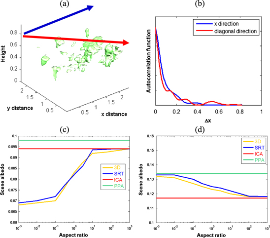
Figure 3. Visualization of a cumulus cloud (a), its horizontal autocorrelation functions along the x and diagonal directions (b). Scene albedos are calculated with various aspect ratios using the 3D Monte Carlo, SRT, PPA, and ICA approaches for 0° (c) and 30° (d) illumination angles.
Download figure:
Standard image High-resolution imageThe third group of simulations are for the stratocumulus cloud system shown in figure 1. The single scattering albedo of cloud droplet is 0.98 and the scattering phase function is the same as the first case. The incidental radiation is collimated light of 0° zenith angle. Boundary conditions are the same as in the first case. The scene albedos calculated using the SRT and the reference 3D Monte Carlo approaches are respectively 0.230 and 0.229, while the cloud absorptance from the SRT and 3D approach is 0.223 and 0.225. The accuracy of the SRT calculation is within 1% of the reference value, while the ICA and PPA result in −5% and 10% errors for this stratocumulus case. It can be seen from these three examples that the magnitude of 3D transport effects varies with many factors, including illumination angle, horizontal fluctuation, and shape of the spatial correlation function (Barker et al 1999).
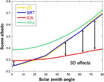
To evaluate if SRT is able to accurately simulate the dependence of radiative fluxes on illumination angle, we computer the reflectance (normalized upward fluxes at the upper boundary) as a function of solar zenith angle. The result for transmittance (normalized downward fluxes at the lower boundary) is not shown here since it complements with reflectance for a non-absorptive medium. It can be seen from figure 4 that, for the checkboard case, the SRT agrees extremely well with the full 3D calculations. The difference between 3D and ICA indicates the magnitude of 3D effects. At small solar angles (<18°), the 3D effects reduce the domain-average reflectance by up to 20%, primarily due to photon leaking from clouds to the clear region. For large solar angles, the 3D effects actually enhance the domain-average reflectance by up to 80%. The enhancement of reflectance increases with solar angle and is mainly due to cloud side illumination effects (Hogan and Shonk 2013). The SRT approach very accurately reproduces the 3D effects for all the examined solar angles.
Figure 4. The scene albedo calculated using different approaches as a function of solar zenith angle. The checkboard cloud case with an aspect ratio of 1 is used to for the simulations.
Download figure:
Standard image High-resolution image
Lastly, the computational cost for the new approach is evaluated and compared with the conventional 1D approaches. To assure fair comparisons, the PPA and ICA approaches also use the same solver as the SRT, in other words,  is set to be
  in equation (2) for the PPA and ICA approaches. The computational cost of the ICA approach is linearly proportional to the number of subcolumns used to represent the horizontal heterogeneity. For the tested cloud cases, the SRT approach is 2–3 times more expensive than the PPA approach while the ICA approach with 100 subcloumns is 30–50 times more expensive than the SRT approach. Depended on the number of photon used in the Monte Carlo simulation, the computational cost of the full 3D approach can be several orders more than the PPA approach.
4. Summary
In this letter a new approach is presented to represent unresolved cloud structure in the radiation parameterization. By using a statistical-physics-like concept, we develop a simple 1D statistical transport theory that naturally utilizes a two-point spatial correlation function to describe subgrid-scale interactions that are traditionally only captured by computationally expensive 3D models. The proposed spatial correlation function encodes the most important information about the spatial arrangement and morphology of clouds and therefore introduces the dependence of radiation field on the 3D structure. Comparison studies of three types of transport media representing checker board, cumulus clouds, and stratocumulus clouds show that the statistical theory is capable of quantitatively capturing the properties of 3D transport models with several orders less computational costs, e.g., enhancement or suppression of reflection by allowing horizontal transport. In practice the 1D stochastic transport transfer approach are expected to lead to a reduction of the computational burden compared to the brute-force Monte Carlo approach, and a significant increase of accuracy compared to the widely used approximation methods. Also noteworthy is that the spatial correlation function appears to be much smoother than the cloud field, indicating that the correlation function should be readily parameterized using point process models or stochastic geometry (Stoyan et al 1995).
It is also important to account for other sources of error such as unresolved temporal variability and spectral resolution in order to develop an accurate cloud radiative transfer parameterization (Pincus and Stevens 2013). Further simplification and evaluation of this approach at other spectral regions and broadband calculations will be the topic of our future work. It should be noted that the new approach developed in this study holds great promise to account for cloud structure in other cloud-related parameterizations.
Acknowledgments
This work is supported by the US Department of Energy's Earth System Modeling (ESM) and Atmospheric Science Research (ASR) programs, and the Laboratory Directed Research & Development program of Brookhaven National Laboratory. We are grateful to Drs Yuri Knyazikhin, Anthony Davis, Warren Wiscombe, and Robert McGraw for their encouragement and insightful advice.