
Abstract
In September 2012, Arctic sea ice cover reached a record minimum for the satellite era. The following winter the sea ice quickly returned, carrying through to the summer when ice extent was 48% greater than the same time in 2012. Most of this rebound in the ice cover was in the Chukchi and Beaufort Seas, areas experiencing the greatest decline in sea ice over the last three decades. A variety of factors, including ice dynamics, oceanic and atmospheric heat transport, wind, and solar insolation anomalies, may have contributed to the rebound. Here we show that another factor, below-average Arctic cloud cover in January–February 2013, resulted in a more strongly negative surface radiation budget, cooling the surface and allowing for greater ice growth. More thick ice was observed in March 2013 relative to March 2012 in the western Arctic Ocean, and the areas of ice growth estimated from the negative cloud cover anomaly and advected from winter to summer with ice drift data, correspond well with the September ice concentration anomaly pattern. Therefore, decreased wintertime cloud cover appears to have played an important role in the return of the sea ice cover the following summer, providing a partial explanation for large year-to-year variations in an otherwise decreasing Arctic sea ice cover.
Export citation and abstract BibTeX RIS

Content from this work may be used under the terms of the Creative Commons Attribution 3.0 licence. Any further distribution of this work must maintain attribution to the author(s) and the title of the work, journal citation and DOI.
1. Introduction
The Arctic is warming at a rate that is approximately twice that of the global average, a phenomenon known as 'Arctic amplification' that has been most pronounced for the Arctic Ocean in autumn and winter over recent decades (Serreze et al 2009, Solomon et al 2007, Serreze and Francis 2006). There has been a dramatic reduction in the observed sea ice extent in the Arctic Ocean (Serreze et al 2007). Model projections suggest a continuation of the warming trend and a decrease in sea ice extent through this century (Holland and Bitz 2003, Zhang and Walsh 2006, Overland and Wang 2013). Nevertheless, year-to-year variations can be large.
The average Arctic sea ice extent in September 2012 was 3.63 million square kilometers; in September 2013 it was 5.35 million square kilometers (National Snow and Ice Data Center, NSIDC), or a 48% increase in the ice extent. Despite this significant rebound, the extent of sea ice in September 2013 was the sixth lowest in the satellite record (NSIDC). Therefore, this was more a return from a prior extreme, and a return to a slower long-term decline, than a recovery to a normal state. Most of this rebound occurred from the East Siberian and Chukchi Seas, where decreases in ice concentration were greatest over the last three decades. What causes this short-term variability?
Various feedback processes, including the ice–albedo feedback and cloud feedbacks (Serreze and Francis 2006, Curry et al 1996) certainly play a role. Clouds have a strong radiative influence on the energy budget at the surface, which controls sea ice growth and melt (Curry et al 1996, Intrieri et al 2002, Liu et al 2008, Tjernström et al 2008). The sensitivity of regional climate to cloud processes is a major uncertainty in projecting changes in the Arctic (Solomon et al 2007). Various satellite-derived products have documented seasonal changes in Arctic cloud amount in recent decades that are associated with measurable impacts on surface energy fluxes (Liu et al 2007, 2008, 2009, Wang and Key 2003, 2005, Schweiger 2004). The Arctic sea ice retreat has also been attributed to the strong role of atmospheric variability, including changes in the Northern Annular Mode (Deser and Teng 2008, Ogi and Rigor 2013), and changes in the Arctic Dipole Anomaly pattern (Overland et al 2012, Wang et al 2009).
Changes in sea ice are very likely to cause changes in cloud cover and other cloud properties (Vavrus et al 2009, 2011, Schweiger et al 2008a, Cuzzone and Vavrus 2011, Kay and Gettelman 2009, Palm et al 2010, Liu et al 2012a). The extent to which clouds influence sea ice cover is less clear. Nussbaumer and Pinker (2012) found that areas showing the largest accumulation of downwelling surface shortwave radiation (total shortwave radiant exposure from the beginning of the year through June) did not correspond to negative sea ice concentration anomalies. Graversen et al (2011) and Kapsch et al (2013) found that years with negative sea ice anomalies correspond to an increase in downwelling longwave radiation during spring from increased cloud cover, which was caused by an anomalous convergence of humid air from lower latitudes.
In contrast, Kay et al (2008) examined the contribution of cloud and radiation anomalies to the 2007 then-record minimum Arctic ice extent and found that increases in downwelling shortwave radiation at the surface resulting from decreases in cloud cover could enhance ice melt by 30 cm or warm the ocean surface by 2.4 K. However, Schweiger et al (2008b) concluded that the negative cloud anomaly and increased downwelling shortwave flux from June through August had no substantial contribution to the record sea ice extent minimum. Kauker et al (2009) claimed that a reduced summer cloud cover has a minor impact, while May and June wind conditions, September 2-meter temperature, and March ice thickness were key to the record-minimum sea ice extent in 2007. Although not addressing cloud cover directly, Perovich et al (2008) concluded that solar heating of the upper ocean was the primary source of heat for the observed enhanced Beaufort Sea bottom melting in the summer of 2007, and therefore a contributor to the record-minimum ice extent.
Most of these studies focused on downwelling shortwave radiation, and none addressed the influence of wintertime cloud and surface radiation anomalies on summertime sea ice extent. The purpose of this paper is to examine Arctic cloud cover and surface radiation in the winter of 2012–2013, its potential effect on ice growth, and how both might have contributed to the significant return in the ice cover during the summer of 2013. It is recognized that other factors may have contributed to variations in the sea ice cover, notably oceanic and atmospheric heat transport and ice dynamics. This study does not attempt to address these factors. Instead, it focuses on the potential effect, and actual effect in the case of 2013, of wintertime cloud cover anomalies on summertime sea ice extent.
2. Data
In this study, Arctic cloud cover is determined primarily with data from the Moderate Resolution Imaging Spectroradiometer (MODIS) onboard the NASA Terra and Aqua satellites. MODIS measures radiances at 36 wavelengths, including infrared and solar bands, with spatial resolutions of 250 m–1 km. Such a robust set of measurements provides the potential for improving cloud detection in the Arctic (Ackerman et al 1998, 2008, Frey et al 2008). While improvements to MODIS cloud detection have been made (Liu et al 2004, Frey et al 2008), there are still larger errors in nighttime Arctic cloud detection than for most other regions on Earth (Holz et al 2008). MODIS data were obtained from the Atmosphere Archive and Distribution System of the NASA Goddard Space Flight Center. Aqua MODIS data for the period 2002–2013 are used here.
Cloud cover from the Cloud-Aerosol Lidar and Infrared Pathfinder Satellite Observation (CALIPSO) (Winker et al 2003) satellite was also examined for comparison to the spatial patterns seen in the MODIS cloud product. The CALIPSO cloud-aerosol lidar with orthogonal polarization (CALIOP) is more sensitive to optically thin cloud layers than MODIS. Because it is an active instrument that is sensitive to small particles, in general, CALIOP has superior cloud detection performance in the polar regions compared to passive satellite instruments like MODIS, especially at night when visible channel information is not available. The CALIPSO Vertical Feature Mask (VFM) from 2006 to 2013 at 5 km resolution (Vaughan et al 2009) is used to calculate the monthly mean cloud amount using approach in Liu et al (2012b). The data were obtained from the Atmospheric Science Data Center of the NASA Langley Research Center.
A daily sea ice concentration product based on the NASA Team algorithm (Cavalieri et al 1996, Maslanik and Stroeve 1999), with brightness temperature data from the Defense Meteorological Satellite Program (DMSP) -F8, -F11 and -F13 Special Sensor Microwave/Imager (SSM/I), and the DMSP-F17 Special Sensor Microwave Imager/Sounder (SSMIS), was obtained from NSIDC. The product was gridded to 25 × 25 km resolution.
The US National Aeronautics and Space Administration (NASA) Modern-era Retrospective Analysis for Research and Applications (MERRA) reanalysis (Rienecker et al 2011) is employed here. MERRA covers the modern era of remotely sensed data, from 1979 through the present. The ECMWF Interim Reanalysis ('ERA-Interim') is also used, primarily as another point for comparison. ERA-Interim is the latest ECMWF global atmospheric reanalysis (Dee et al 2011). The ERA-Interim project replaces the previous atmospheric reanalysis ERA-40. It also covers the period 1979 through the present. Reanalysis variables of interest here include cloud cover (total, low-, mid-, and high-level), surface radiation, surface temperature, geopotential height, and vertical pressure velocity at 500 hPa (OMEGA500). Both reanalyses give similar results in this study, so results are presented mainly for MERRA. Significant differences between the two are noted.
Other datasets employed in this study include preliminary sea ice thickness estimates based on the European Space Agency's CryoSat-2 satellite from the Alfred Wegener Institute (unpublished data; www.meereisportal.de/cryosat), sea ice motion vectors from the Polar Pathfinder daily, 25 km EASE-Grid product (Fowler et al 2013), and ice thickness observations from the NASA IceBridge aircraft campaign available from NSIDC (2012).
3. Winter 2013 cloud amount
In January of 2013, Aqua MODIS showed negative cloud cover anomalies compared to the 2002–2012 mean over most area of the Beaufort Sea, Chukchi Sea, Canada Basin, Central Arctic, and the Laptev Sea, extending to north central Russia over land (figure 1). The negative anomalies are approximately −20%. The actual monthly mean cloud amount over some of these regions is less than 20% in that month. A similar anomaly pattern can be seen in CALIPSO data for January 2013 compared to the 2006–2013 mean, and also in the MERRA reanalysis (figure 1). The 2013 January cloud amount anomalies over the Arctic Ocean from MODIS and MERRA are larger than two standard deviations of the monthly mean cloud amount from 2002 to 2012. With regard to remote sensing accuracy, MODIS detects less cloud than active satellite lidar/radar sensors over ice, and this difference increases with increased sea ice concentration (Liu et al 2010). This is not an issue in our analysis because there are no significant sea ice concentration changes over these regions in January and February in the regions of interest. A significant negative sea ice concentration trend, on the other hand, would lead more cloud detected, not less.
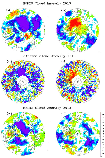
Figure 1. Cloud cover anomalies (%) in (a) January and (b) June 2013 from Aqua MODIS, in (c) January and (d) June 2013 from CALIPSO, and in (e) January and (f) June 2013 from the MERRA reanalysis. The anomalies are calculated relative to the monthly means for the periods 2002–2012, 2006–2013, and 2002–2012 for Aqua MODIS, CALIPSO, and MERRA, respectively.
Download figure:
Standard image High-resolution imageThe January 2013 cloud amount anomaly pattern corresponds to a positive geopotential height anomaly over the same region (figure 2). This anomalously high pressure system may be the cause of the negative cloud amount anomaly. Positive wintertime geopotential height anomalies generally result in less cloud cover (Liu et al 2007, 2008). This is confirmed in the MERRA reanalysis, where anomalously high 850 hPa geopotential height over the Arctic Ocean corresponds to the negative anomalies in the total cloud amount. The anomalies of vertical pressure velocity at 500 hPa indicate stronger downward air motion over the region of negative cloud cover anomalies (figure 2).
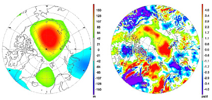
Figure 2. The 850 hPa geopotential height anomalies (unit: m; left) from MERRA and the 500 hPa omega anomalies (unit: (Pa/100)/day; right) for January 2013 from MERRA. The anomalies are calculated relative to the 2002–2012 mean for the month.
Download figure:
Standard image High-resolution imageIn February, the anomalously high pressure system seen in January becomes weaker and moves southward from the North Pole (not shown). The negative anomaly in total cloud amount becomes most apparent near the coastal area of Beaufort, Chukchi Seas, and the northeastern Russia in MODIS data. This February anomaly is larger than one standard deviation of the monthly mean cloud amount from 2002 to 2012. CALIPSO shows a more extensive distribution of negative cloud amount anomaly over the Arctic Ocean but a similar magnitude overall.
ERA-Interim total cloud cover also shows a negative anomaly over the Canada Basin, but positive anomalies over the Laptev Sea and the region north of Greenland in January (figure 3). In February, a negative anomaly appears over part of the Beaufort Sea, with positive anomalies over other parts of the Arctic Ocean. Low-level clouds, located between the 0.8 and 1.0 model sigma levels, show similar anomaly patterns. For the medium-level cloud, lying between the 0.45 and 0.80 sigma levels, the anomaly distribution and magnitude are similar to those of MODIS Aqua and CALIPSO (figure 1). Medium-level cloud cover in the ERA-Interim data therefore corresponds closely to the satellite-derived cloud patterns.

Figure 3. Cloud cover anomalies (%) in (a) January and (b) June 2013, and medium cloud cover anomalies (%) in (c) January and (d) June 2013 from the ERA-Interim reanalysis. The anomalies are calculated relative to the monthly means for the periods 2002–2012.
Download figure:
Standard image High-resolution imageThe anomalously high pressure pattern remained over the Arctic Ocean through March. However, there is no anomalously low cloud amount seen in either MODIS or CALIPSO in March over most of the Arctic Ocean except over part of the Beaufort Sea, suggesting that large-scale circulation may not be the only cause of cloud cover anomalies in the Arctic.
4. Cloud radiative effect and surface energy budget
Clouds affect the surface energy budget through changes in downwelling shortwave and longwave radiation. The cloud radiative effect, or 'forcing', is the net radiation flux difference under the cloudy and clear conditions. Cloud forcing is the integrated partial derivative of the radiative flux with respect to the cloud fraction and is defined as


where CS, CF, and CNET are the shortwave, longwave, and net cloud forcing for the surface (subscript s), Ac is the total cloud amount, Ss and Fs are the net shortwave and longwave fluxes at the surface, and a is the cloud fraction. Cloud forcing is negative for cooling and positive for warming. The net cloud forcing is the sum of shortwave and longwave cloud forcing.
Clouds have a warming effect on the surface most of the year in the Arctic except in the summer (Intrieri et al 2002, Schweiger and Key 1994, Stone 1997). Stone et al (2005) showed that at Barrow, Alaska during February, a 5% increase in cloud cover produced an increase in surface temperature of 1.4 °C on average over a 33-year period. The below-average cloud amount in January and February 2013 will therefore have a cooling effect on the surface.
The cloud radiative forcing at the surface calculated from the MERRA and ERA-Interim data shows negative anomalies over most Arctic Ocean in January 2013 (figures 4 and 5), and over part of the Chukchi, and Beaufort Seas in February 2013. The anomaly pattern corresponds well to the cloud cover anomalies in MODIS CALIPSO, and MERRA data. This indicates that less cloud cover in January and February does, in fact, have a cooling effect on the surface. It also suggests that this effect may result primarily from a negative anomaly in ERA-Interim medium-level cloud cover for this particular case.
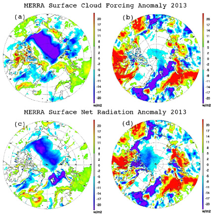
Figure 4. MERRA surface net cloud forcing anomalies for (a) January and (b) June, and the surface net radiation anomalies for (c) January and (d) June relative to the 2002–2012 mean.
Download figure:
Standard image High-resolution image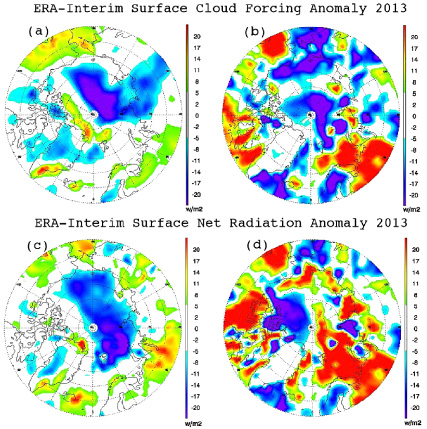
Figure 5. ERA-Interim surface net cloud forcing anomalies for (a) January and (b) June, and the surface net radiation anomalies for (c) January and (d) June relative to the 2002–2012 mean.
Download figure:
Standard image High-resolution imageTo further verify the modeled cloud radiative forcing from MERRA, estimates were made with CALIPSO cloud cover. The monthly mean cloud radiative forcing over 75–90°N of Key et al (1999, also shown in Intrieri et al 2002, figure 12), which is a update of Schweiger and Key (1994), was used. The product of this monthly mean cloud radiative forcing and the ratio of the January 2013 CALIPSO cloud amount anomaly to the monthly mean cloud amount over the period 2006–2013 gives an estimate of the actual January cloud radiative forcing anomaly. The derived cloud radiative forcing from January to March is similar to the MERRA cloud radiative forcing in both spatial distribution and magnitude. The cloud radiative forcing from both MERRA and CALIPSO is lower than − 20 W m−2 over of the Arctic Ocean in areas of negative cloud cover anomalies.
The surface radiation budget is strongly controlled by cloud cover and has the same spatial pattern as that of cloud forcing. Figures 4 and 5 show the surface net radiation budget anomaly for January and June. The decreased wintertime net radiation and thus cooling has been confirmed by measurements at the NOAA Baseline Observatory, Barrow, Alaska, where the surface radiation budget has been monitored for many years. During January 2013, for instance, there was a reduction in net radiation at the surface of approximately 12 W m−2, which is consistent with the MERRA and ERA-Interim reanalyses for that location.
5. Influence of cloud cover anomalies on summertime sea ice return
Negative surface cloud radiative forcing and net radiation anomalies favor sea ice growth. Thorndike (1992) presented a simple method to relate a change in ice thickness to surface net radiation:

where t is length of the time period, ρ is the density of sea ice (917 kg m−3), L is the latent heat of fusion for sea ice (333.4 kJ kg−1), Fs is net longwave radiation at surface, Ss is net shortwave radiation at surface, and FW is the conductive heat flux at the ice–ocean interface. This equation is similar to (1) in Eisenman et al (2007). To isolate the cloud forcing effect on ice growth, this equation can be rewritten as

where Fnet(0) is surface net radiation for clear sky and CNETs is the surface net cloud radiative forcing. The turbulent surface fluxes of sensible and latent heat and the conductive flux are neglected, as they are much smaller than the radiative fluxes. This is a limitation of the model, one that introduces some error. For example, the conductive heat flux is likely to decrease with increased ice thickness, so that ice growth will be smaller for thicker sea ice with the same cloud radiative forcing. Surface emissivity, albedo, and the conductive heat flux are functions of snow depth, and uncertainty in the snow depth would also lead to some error in the sea ice growth estimates.
Using the relatively simple above method, 1 W m−2 of negative monthly net cloud radiative forcing anomaly would theoretically grow 0.85 cm of sea ice. Sea ice growth resulting from the January–February 2013 negative cloud radiative forcing anomaly is shown in figure 6 based on cloud radiative forcing from MERRA. Results using the estimated CALIPSO cloud forcing are similar. Sea ice growth up to 45 cm more occurs over the western Arctic Ocean in January and February, the same area with the greatest sea ice return the following summer.

Figure 6. (a) Ice growth estimated from MERRA net cloud radiative forcing in January and February 2013, where white represents land areas and areas with sea ice concentration less than 15% in March 2013. (b) Ice thickness distribution at the beginning of September due to ice drift, where white represents areas with sea ice drifted away. (c) Sea ice concentration anomalies for September 2013 from SSMIS observations relative to the 2002–2012 mean.
Download figure:
Standard image High-resolution imageThe two anomalous areas of sea ice growth and sea ice concentration in figure 6 do not match exactly. The discrepancy can be partially explained by ice drift. The mean annual Arctic sea ice motion is characterized by two primary features: the Beaufort Gyre and the Transpolar Drift Stream; the winter pattern is similar (Serreze and Barry 2005). Sea ice motion vectors in 2013 from the Polar Pathfinder daily, 25 km EASE-Grid product (Fowler et al 2013) were used to move the initial sea ice growth anomaly field in figure 6(a). After applying the ice motion field from the end of February 2013 to the beginning of September, the final, 'drifted' ice growth anomaly field is shown in figure 6(b). At the beginning of September, the extra ice growth from January–February that resulted from cloud radiative cooling, advected with sea ice drift data, is significant over the Beaufort Sea and Chukchi Seas. This corresponds to the anomalously high sea ice concentration over those regions in September (figure 6(c)). The drifted ice accumulation is also high over the Laptev Sea, though the September sea ice concentration anomaly in that area is mostly negative. Other processes, such as ocean heating, freshwater influx, and solar insolation may be controlling factors in that area.
Ice thickness observations in March 2012 and March 2013 are available from the NASA IceBridge aircraft campaign. The same flight routes over the Beaufort Sea were chosen for 2012 and 2013. Relative frequency distributions of the in situ ice thickness observations were derived (figure 7). Though the mean sea ice thicknesses in 2012 (1.84 m) and in 2013 (1.81 m) are comparable, the distributions show a lower frequency of sea ice with thicknesses less than 1 m in 2013 than in 2012, a greater frequency of ice with thicknesses between 1 and 2.5 m in 2013, and a marginally lower frequency of ice thicker than 2.5 m in 2013. Overall, there is 6% more sea ice thicker than 1.5 m in 2013 than in 2012. This finding supports, but does not prove, the hypothesis that below-average January–February 2013 cloud cover led to greater ice growth. It also helps explain why ice cover in those regions persisted through the summer. On a broader spatial scale, the March 2012 and 2013 ice thickness differences from IceBridge data have been confirmed with ice thickness estimates from the European Space Agency's CryoSat-2 satellite. CryoSat-2 is a radar altimeter that measures sea ice freeboard. Preliminary sea ice thickness estimates from the Alfred Wegener Institute show positive ice thickness differences (March 2013 minus March 2012) over most of the Beaufort, and Chukchi Seas (figure 7). The CryoSat-2 ice thicknesses also indicate that the ice grew more from January to March in the East Siberian and Beaufort Seas in 2013 than in 2012. Furthermore, the ice thickness data show substantial ice growth between December 2012 and March 2013 (figure 8) in the areas of large cloud forcing (figure 6(a)), though the simple ice growth model and cloud forcing cannot explain the growth in other areas.
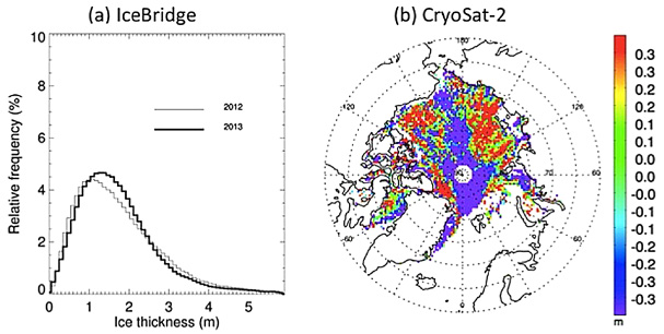
Figure 7. (a) Ice thickness probability distribution function in 2012 (thin line) and in 2013 (thick line) based on data from IceBridge flights north of Alaska. (b) Difference in ice thickness in March 2013 and March 2012 based on CryoSat-2 satellite altimeter data.
Download figure:
Standard image High-resolution image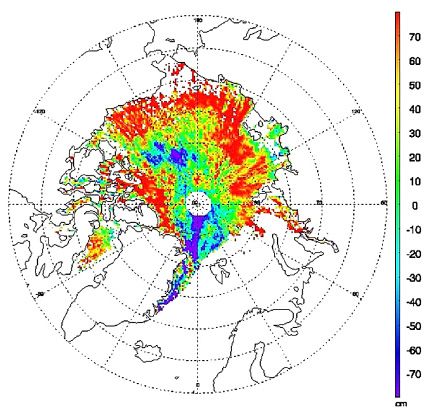
Figure 8. Difference in ice thickness in between December 2012 and March 2013 (March minus December thickness) based on CryoSat-2 satellite altimeter data.
Download figure:
Standard image High-resolution image
Chevallier and Salas-Mélia (2012) suggest that sea ice area anomalies in August and September are potentially predictable from the area covered by sea ice thicker than 0.9–1.5 m as much as 6 months in advance. In September of 2013, sea ice concentration is anomalously high over the Beaufort and Chukchi Seas (figure 6). These areas are, for the most part, the same areas that theoretically would have the most growth as a result of the lower January–February cloud amounts, and the areas that were observed to have anomalously thick ice in March.
In June a positive cloud amount anomaly appears from the Beaufort Sea to the Chukchi Sea in MODIS data (figure 1), which is expected to lead to decreased net shortwave radiation due to the cloud reflection and increased longwave radiation at the surface. However, it is not clear whether or how this cloud anomaly in the early summer contributes to sea ice extent in September considering previous work by others on summertime solar radiation effects on sea ice anomalies (cf, Kay et al 2008, Schweiger et al 2008b, Kauker et al 2009). The positive cloud amount anomaly seen in the satellite data is not apparent in the MERRA or ERA-Interim reanalyses. The air surface temperature anomaly over the Beaufort and Chukchi Seas is near zero, as was the surface net radiation anomaly. However, below-average net surface radiation occurs northwest of the Canadian Arctic Archipelago (figures 4(d), 5(d)) as well as the relatively low air temperature (Overland et al 2013), where downwelling solar radiation is reduced by cloud cover. Overall, the cloud radiative effect on the surface energy budget is larger in January than in June.
6. Summary and conclusions
The recent observed decline in Arctic sea ice extent involves a variety of climate processes (Serreze et al 2007, Francis et al 2009, Stroeve et al 2012), including large-scale circulation, ocean currents, radiative fluxes, surface air temperature, and sea ice dynamics. Wind associated with the large-scale circulation is very likely to re-distribute the sea ice thickness field in the wintertime. Anomalies in air temperature over the ocean and northern lands affect the sea ice melt rate. The role of clouds and their radiative effects on sea ice cover, however, is not well understood. Previous studies of summertime clouds, solar insolation, and sea ice anomalies have yielded inconsistent, if not contradictory, results (cf, Nussbaumer and Pinker 2012, Kapsch et al 2013, Graversen et al 2011, Kay et al 2008, Schweiger et al 2008b, Kauker et al 2009). Here we focused on wintertime clouds, demonstrating that anomalous cloud cover can have a significant influence on summertime sea ice cover.
In September 2012, Arctic sea ice cover reached a record minimum for the satellite era. In contrast, a year later the Arctic sea ice extent was 48% greater than the same time in 2012. Nevertheless, the extent of sea ice in September 2013 was still the sixth lowest in the satellite record (NSIDC). Most of this return from a previous extreme was in the Chukchi and Beaufort Seas, areas that have experienced the greatest decline in sea ice over the last three decades. What factors contributed to this rebound, and what processes cause large interannual variations in an otherwise declining sea ice cover?
An examination of wintertime cloud amount with two satellite products and climate model reanalysis data showed below-average cloud cover in January–February 2013 over most of the Arctic Ocean. The cloud cover anomalies correspond well with above-average 850 hPa geopotential height and anomalous downward atmospheric motion, implying that large-scale circulation was the cause of the below-average cloud cover. Less cloud in the Arctic winter results in a more strongly negative surface radiation budget, cooling the surface and allowing for greater ice growth. The cloud radiative effect was verified by satellite estimates and by climate reanalysis data.
Ice growth resulting from the wintertime cloud radiative forcing was theoretically estimated to be as much as 45 cm. Thicker ice in March 2013 relative to March 2012 in the western Arctic Ocean was, in fact, observed in ice thickness estimates from aircraft and satellite, and spatial patterns of satellite-derived ice thickness corresponded qualitatively to the cloud cover, cloud radiative forcing, and surface net radiation anomalies. Areas of estimated ice growth that resulted directly from the negative cloud forcing anomalies in January–February were allowed to drift based on ice motion fields from March to August. The advected sea ice growth anomaly pattern corresponds well with ice concentration anomalies over the Beaufort Sea and Chukchi Seas at the beginning of September. Therefore, decreased cloud cover in the early winter of 2013 appears to have played an important role in the return of sea ice in the summer of 2013. Furthermore, positive cloud cover anomalies in June 2013 may have a cooling at the surface. In itself, this would help maintain the ice cover. In other months of 2013, there do not appear to be significant basin-scale changes in cloud amount over the Arctic Ocean.
Changes in cloud cover associated with large-scale circulation changes can have a significant impact on the surface radiation budget, and are likely to influence the sea ice growth and melt. Many factors may lead to ice thickness changes in the winter, e.g. the atmospheric heat advection and oceanic currents. Here, we demonstrated that anomalous cloud cover in winter 2013 likely contributed to increased ice thickness, which in turn affected the summertime sea ice area. Cloud cover anomalies, therefore, can contribute significantly to large year-to-year sea ice cover variations, and can affect the accuracy of summer sea ice cover predictions.
Future work will examine the role of clouds for other cases over the last decade when the Arctic sea ice cover has changed significantly from one year to the next. While there may be instances where variability in cloud cover had a significant influence on ice extent, the complexity of the climate system ensures that other factors and relationships will often dominate.
Acknowledgments
This work was supported by the NOAA National Climatic Data Center (NCDC) and the Joint Polar Satellite System (JPSS) Program Office. We are grateful to the German CryoSat Office of the Alfred Wegener Institute (www.meereisportal.de/cryosat) for providing their preliminary ice thickness estimates to the scientific community for evaluation. We thank R Stone for valuable discussions on this work, and for his analysis of data from the NOAA Baseline Observatory at Barrow. We also thank M Tschudi for providing the 2013 Polar Pathfinder daily 25 km EASE-Grid sea ice motion data. The MODIS data used in this study were acquired as part of the NASA's Earth–Sun System Division and archived and distributed by the MODIS Adaptive Processing System (MODAPS). The CALIPSO data were obtained from the NASA Langley Research Center Atmospheric Science Data Center. The views, opinions, and findings contained in this report are those of the author(s) and should not be construed as an official National Oceanic and Atmospheric Administration or US Government position, policy, or decision.