
Abstract
Several papers reported associations between airborne fine particulate matter (PM2.5) and birth weight, though findings are inconsistent across studies. Conflicting results might be due to (1) different PM2.5 chemical structure across locations, and (2) various exposure assignment methods across studies even among the studies that use ambient monitors to assess exposure. We investigated associations between birth weight and PM2.5 chemical constituents, considering issues arising from choice of buffer size (i.e. distance between residence and pollution monitor). We estimated the association between each pollutant and term birth weight applying buffers of 5 to 30 km in Connecticut (2000–2006), in the New England region of the USA. We also investigated the implication of the choice of buffer size in relation to population characteristics, such as socioeconomic status. Results indicate that some PM2.5 chemical constituents, such as nitrate, are associated with lower birth weight and appear more harmful than other constituents. However, associations vary with buffer size and the implications of different buffer sizes may differ by pollutant. A homogeneous pollutant level within a certain distance is a common assumption in many environmental epidemiology studies, but the validity of this assumption may vary by pollutant. Furthermore, we found that areas close to monitors reflect more minority and lower socio-economic populations, which implies that different exposure approaches may result in different types of study populations. Our findings demonstrate that choosing an exposure method involves key tradeoffs of the impacts of exposure misclassification, sample size, and population characteristics.
Export citation and abstract BibTeX RIS

Content from this work may be used under the terms of the Creative Commons Attribution 3.0 licence. Any further distribution of this work must maintain attribution to the author(s) and the title of the work, journal citation and DOI.
Introduction
Research generally indicates associations between gestational exposure to air pollution and adverse birth outcomes, although findings are inconsistent. For instance, particulate matter with aerodynamic diameter ≦̸2.5 μm (PM2.5) was associated with birth outcomes in California, but not in Oslo, Norway [1–3]. Although results vary, several reviews concluded that weak to moderate associations exist between PM2.5 and birth outcomes [4–6].
One potential explanation for inconsistent results is substantial variation in PM2.5's chemical structure by location, which may affect toxicity. For instance, PM2.5 sulfate (SO4) levels are higher in the eastern US, with higher PM2.5 nitrate (NO3) levels in the west [7]. A limited number of studies explored PM2.5 chemical constituents with birth outcomes. Elemental carbon (EC) was associated with lower birth weight in Atlanta [8]. In the New England region of the US, aluminum (Al), EC, nickel (Ni), potassium (K), silicon (Si), titanium (Ti), vanadium (V), and zinc (Zn) were linked to lower birth weight [9–11]. In California, lower birth weight was associated with ammonium ion (NH4+), bromine, copper, EC, iron, manganese, SO4, sulfur, Ti, V, and Zn [12]. The US Environmental Protection Agency (EPA) identified study of health associations of particle chemical constituents as a critical research need [13].
Another possible explanation is the variation in exposure methods. Typically, air pollution exposure is estimated by: (1) assigning measurements from the nearest monitor within a certain distance (i.e. buffer) from residence [14], (2) averaging or interpolating values from monitor(s) within geographic unit(s) (e.g. county) [15], or (3) combining alternative sources (e.g. traffic, satellite) and/or monitor data to predict concentrations at a given point or area [16]. These methods were applied in many studies to estimate exposure based on residence (e.g. mother's actual address or residential county at birth) [17–21]. Applying large buffers (or spatial units) can introduce exposure misclassification due to spatial heterogeneity of pollution [22]. However, applying small buffers (or spatial units) can limit sample size and lower statistical power. Furthermore, EPA monitors tend to be located in urban environments [12]. Because people with low socio-economic status (SES) are more likely to live in urban environments in the US, small buffers might exclude sub-urban and rural persons, resulting in different populations than would be selected with larger buffers. In fact, literature reviews identify exposure assignment as a key challenge in air pollution and birth outcomes research [4–6].
Buffer sizes for air pollution can vary from a few to 50 km [23, 24]. Researchers generally select these distances based on previous studies or assumptions of reasonable values, but typically do not systematically address variation in spatial heterogeneity by pollutant [8, 25]. This raises questions regarding how well estimated exposures represent actual exposures and creates challenges for comparisons across studies.
A few studies compared results under various exposure assignments with inconsistent results. Third trimester particulate matter with aerodynamic diameter ≦̸10 μm (PM10) exposure was associated with low birth weight (LBW: birth weight <2500 g) for mothers living ≦̸1 mi (1.6 km) from monitors, with no associations using buffers >1 mi in Los Angeles [26]. In contrast, PM10 and PM2.5 associations for birth weight were comparable under buffers of 5, 10, and 20 km, and county-based assignment in North Carolina [27]. Questions remain regarding the implications of buffer size given pollutants' different spatial heterogeneity. In particular, few studies have explored the impacts of choice of buffer size on health associations for PM2.5 chemical constituents. Patterns of surface concentrations can differ by PM2.5 constituents, with some showing relative spatial homogeneity at long distances, while others exhibit spatial heterogeneity within short distances [22].
We investigated associations between PM2.5 and PM2.5 chemical constituents and birth weight in Connecticut, in the New England region of the US. We address limitations of previous studies [9–11, 28] by investigating: (1) whether effects differ by chemical constituents, in addition to estimating associations for PM2.5 total mass; and (2) implications of different buffer sizes to assign exposure. Previously, exposure was estimated based on mother's county of residence, whereas here we benefited from detailed birth certificates that include exact mothers' residence. Furthermore, we analyzed whether associations differ by neighborhood SES (e.g. poverty level). Luo et al found that adverse birth outcomes were associated with lower SES neighborhoods in addition to lower individual SES [29]. Our previous studies could not control for neighborhood-level SES due to lack of exact residence. To date, no previous studies evaluated choice of PM2.5 constituents' buffer size on health associations in the Northeastern US, which is more densely urbanized and has different pollutant composition than other US regions.
Methods
Birth data
Birth certificate data (1 January 2000–31 December 2006) were obtained from the Connecticut Department of Public Health. Data contain information of infants and parents (e.g. birth weight, gestational age). Unlike birth certificate data that are publically available, these data have residential address at birth and exact date of birth. We obtained neighborhood SES by identifying residential census tracts (average size 120.5 km2 in Connecticut). Specifically, we obtained three neighborhood-related variables from American Community Survey: percentage of educational attainment less than a high school degree for population ⩾25 years (S1501 (American Community Survey 2009)), percentage of population with income below the poverty level (S1701), and percentage of unemployed for population ⩾16 years (S2301) [30].
There were 288 635 births in Connecticut in the study period. We excluded from analysis infants with gestational age <37 weeks (non-term births) or >44 weeks (n = 19 838 (6.9%)). We also excluded births with plural deliveries (12 119 (4.2%)), confirmed congenital defects (2406 (0.8%)), mothers with acute or chronic lung disease or pre-existing diabetes (2868 (1.10%)), unknown infants' sex (3 (0.001%)), birth weight <1000 g or >5500 g (1586 (0.5%)), or impossible gestational age and birth weight combinations (98 (0.03%)) [31]. Similar criteria were applied in earlier studies [9, 28]. Births were also excluded if mother's address at birth was missing (1848 (0.6%)) or gestational age was missing (157 (0.05%)). Some subjects were excluded for multiple criteria. After applying exclusion criteria, 39 039 (13.5%) subjects were excluded from the original data, leaving 249 596 births.
Air pollution and weather data
Ambient monitoring data from EPA were used to estimate gestational pollutant exposures for PM2.5 total mass and selected PM2.5 chemical constituents: Al, NH4+, calcium (Ca), chlorine (Cl), EC, Ni, NO3, organic carbon matter (OCM), Si, sodium ion (Na+), SO4, Ti, V, and Zn [32, 33]. Previous studies explored these PM2.5 constituents in relation to health [28, 34–36]. Measurement frequency was typically every three to six days. Data were restricted to Connecticut and surrounding areas from 1999 to 2006 for PM2.5 total mass, and from 2000 to 2006 for PM2.5 chemical constituents, as most constituent monitoring sites began sampling in 2000. Supplemental figure 1 shows monitor locations.
To incorporate associations of weather on birth weight, apparent temperature (AT) was included in the model, similar to previous studies [28]. Taking account for temperature and humidity, AT is designed to address overall weather discomfort [37]. Data from six weather monitors in Connecticut and surrounding areas were available from the National Climatic Data Center. We assigned values from the closest weather monitor from each residence.
Exposure estimation
Daily pollutants levels were assigned for those who live within a certain distance from monitors: we explored buffer size of 5, 10, 15, 20, 25, and 30 km, which are equal to 3.1, 6.2, 9.3, 12.4, 15.5, and 18.6 mile, respectively. Using these pollutant levels, we first calculated weekly pollutant levels and then estimated an average exposure from conception date to delivery date (i.e. gestation) for each birth and each pollutant. Gestational exposure was defined based on birth date and gestational age, which was obtained from ultra sound, or birth date and last menstrual period if gestational age was not available, assuming conception date as two weeks after last menstrual period. We excluded births for which weekly exposure estimates were unavailable for >25% of weeks in any trimester for the pollutant to protect against biases due to differences in measurement frequency. If the residence was within the buffer from multiple monitors, we first estimated gestational exposures based on each monitor, and then calculated an inverse distance weighted average of those values. This approach was repeated for each birth and pollutant for various buffer sizes: 5, 10, 15, 20, 25, and 30 km.
As an alternative way, we estimated county-based gestational exposures for each pollutant, which many papers applied previously [11, 15]. Daily pollutant levels were assigned for each birth based on the county of residence, rather than a specified buffer. In cases with multiple monitors within the county, we averaged across monitors' values for each day. Gestational exposures were calculated for each birth in same manner described above.
For each individual, we calculated average AT exposure for each trimester using the nearest monitor. Trimesters were defined as 1–13weeks, 14–26 weeks, and week 27 to delivery [28].
Statistical analysis
To estimate the pollutants' associations with birth weight, gestational exposure to each pollutant was regressed against birth weight as a continuous variable. The model was adjusted by infant's sex, gestational age, birth order, the trimester prenatal care began, maternal age, maternal race, maternal education, mother's marital status, mother's alcohol consumption during entire pregnancy, mother's smoking during entire pregnancy, season of birth, indicator variable for year of birth, three neighborhood SES variables, and AT for each trimester. Except neighborhood SES, pollution, and AT, all variables were obtained from birth certificate data. Earlier work on air pollution and pregnancy outcomes used similar methodology [8, 9]. For each pollutant, separate models were fit for each buffer size and county-based exposure.
Several sensitivity analyses were conducted. First, logistic regressions were fitted for all buffer sizes (5–30 km) and county-based exposure, using LBW as an outcome. Second, two pollutant linear regression models were conducted using birth weight as an outcome for pollutants that showed associations with a 30 km buffer. This analysis aims to explore the robustness of associated pollutants with adjustment by an additional pollutant. Adjusted pollutants were selected only when the pair of pollutants were not highly correlated (correlation <0.5). Third, trimester-specific effects were explored with 30 km buffer. Specifically, trimester exposures were put in linear regression models simultaneously. Given that trimester exposures are likely correlated, we used estimates of trimester exposures that were adjusted for exposures of other trimesters. Further description of the method used for trimester analysis is described elsewhere [28].
Studies in the US found that monitors are more common in urban and lower SES areas [12, 38]. Given that choice of buffer size may affect characteristics of the study population, we investigated population characteristics in relation to distance from monitors. We created a 30 km buffer for each monitor, and divided it into three areas: 10 km buffer, area between 10 km and 20 km buffers (10–20 km ring), and area between 20 km and 30 km buffers (20–30 km ring) (supplemental figure 2). We compared the distribution of population characteristics for each area (10 km buffer, 10–20 km ring, 20–30 km ring).
Results
Population characteristics and exposures
Among the 249 596 subjects who met our inclusion criteria, 17 673 subjects were born to mothers living >30 km from any monitor, and were excluded. Of these, 70% are from Middlesex County, which had no monitors, or New London County, where monitors started measuring after 2003 (supplemental figure 1). The sample size of subjects for each buffer size and pollutant is available in table 1. The number of births increases as buffer size increases. For instance, the number of subjects for PM2.5 aluminum with 30 km buffer (n = 30 228) was about nine times larger than with a 5 km buffer (n = 3254). Furthermore, the number of births differs by pollutant, with more subjects for PM2.5 total mass than PM2.5 chemical constituents, due to differences in the monitoring networks. There were 25 monitors available for PM2.5 total mass, with 6 for PM2.5 chemical constituents (supplemental figure 1). Table 1 also presents the sample size for analysis using county-based exposures, which was generally larger than the sample size for the 25 km buffer, but smaller than that of the 30 km. The area of the counties ranged from 990 to 2446 km2 and averaged 1607 km2.
Table 1. Summary of gestational exposures to pollutants and interquartile values based on the 5 km–30 km buffers, and county-based assignmenta.
| 5 km Buffer | 10 km Buffer | 15 km Buffer | 20 km Buffer | 25 km Buffer | 30 km Buffer | County based | ||||||||||||||||
|---|---|---|---|---|---|---|---|---|---|---|---|---|---|---|---|---|---|---|---|---|---|---|
| Pollutants | Number of births | Mean exposure level (standard deviation) | IQR | Number of births | Mean exposure level (standard deviation) | IQR | Number of births | Mean exposure level (standard deviation) | IQR | Number of births | Mean exposure level (standard deviation) | IQR | Number of births | Mean exposure level (standard deviation) | IQR | Number of births | Mean exposure level (standard deviation) | IQR | Number of births | Mean exposure level (standard deviation) | IQR | |
| PM2.5 Total mass (μg m−3) | 75 034 | 12.8 (1.3) | 1.61 | 122 455 | 12.7 (1.4) | 1.74 | 162 533 | 12.6 (1.4) | 1.74 | 199 551 | 12.5 (1.4) | 1.79 | 219 323 | 12.4 (1.4) | 1.79 | 230 640 | 12.4 (1.4) | 1.76 | 214 446 | 12.6 (1.7) | 2.25 | |
| PM2.5 Chemical constituents (μg m−3) | Aluminum | 3254 | 0.018 (0.005) | 0.0072 | 6311 | 0.017 (0.005) | 0.0074 | 9493 | 0.016 (0.005) | 0.0072 | 14 355 | 0.016 (0.005) | 0.0070 | 19 852 | 0.016 (0.005) | 0.0069 | 30 228 | 0.016 (0.005) | 0.0070 | 25 578 | 0.016 (0.005) | 0.0056 |
| Ammonium Ion | 4607 | 1.52 (0.17) | 0.21 | 8606 | 1.49 (0.19) | 0.25 | 11 273 | 1.47 (0.20) | 0.31 | 15 776 | 1.45 (0.21) | 0.35 | 21 059 | 1.45 (0.22) | 0.35 | 32 008 | 1.47 (0.22) | 0.32 | 25 413 | 1.49 (0.21) | 0.34 | |
| Calcium | 3254 | 0.031 (0.003) | 0.0034 | 6311 | 0.030 (0.003) | 0.0037 | 9493 | 0.029 (0.004) | 0.0060 | 14 355 | 0.028 (0.005) | 0.0070 | 19 852 | 0.028 (0.006) | 0.0078 | 30 228 | 0.029 (0.010) | 0.0082 | 25 578 | 0.028 (0.005) | 0.0077 | |
| Chlorine | 3254 | 0.017 (0.009) | 0.0086 | 6311 | 0.016 (0.009) | 0.0084 | 9493 | 0.014 (0.010) | 0.0096 | 14 355 | 0.013 (0.010) | 0.0090 | 19 852 | 0.013 (0.010) | 0.0090 | 30 228 | 0.013 (0.011) | 0.0101 | 25 578 | 0.017 (0.014) | 0.0167 | |
| Elemental carbon | 4642 | 0.878 (0.104) | 0.13 | 8710 | 0.857 (0.127) | 0.13 | 11 979 | 0.814 (0.174) | 0.16 | 17 339 | 0.784 (0.195) | 0.28 | 23 851 | 0.767 (0.218) | 0.30 | 36 389 | 0.785 (0.231) | 0.30 | 37 245 | 0.767 (0.219) | 0.30 | |
| Nickel | 3254 | 0.006 (0.001) | 0.0019 | 6311 | 0.006 (0.002) | 0.0024 | 9493 | 0.005 (0.002) | 0.0048 | 14 355 | 0.004 (0.002) | 0.0048 | 19 852 | 0.004 (0.003) | 0.0048 | 30 228 | 0.005 (0.005) | 0.0049 | 25 578 | 0.004 (0.002) | 0.0045 | |
| Nitrate | 4666 | 1.38 (0.20) | 0.26 | 8784 | 1.36 (0.21) | 0.28 | 12 524 | 1.28 (0.30) | 0.35 | 18 397 | 1.24 (0.34) | 0.37 | 25 160 | 1.22 (0.36) | 0.41 | 38 347 | 1.24 (0.39) | 0.42 | 30 878 | 1.25 (0.39) | 0.44 | |
| Organic carbon matter | 4560 | 3.61 (0.36) | 0.51 | 8516 | 3.58 (0.37) | 0.50 | 11 157 | 3.55 (0.38) | 0.49 | 15 666 | 3.52 (0.39) | 0.48 | 21 239 | 3.51 (0.42) | 0.50 | 32 364 | 3.54 (0.45) | 0.54 | 30 607 | 3.49 (0.37) | 0.46 | |
| Silicon | 3254 | 0.054 (0.010) | 0.010 | 6311 | 0.056 (0.011) | 0.011 | 9493 | 0.060 (0.016) | 0.014 | 14 355 | 0.062 (0.018) | 0.015 | 19 852 | 0.062 (0.020) | 0.016 | 30 228 | 0.063 (0.020) | 0.017 | 25 578 | 0.063 (0.018) | 0.013 | |
| Sodium ion | 4607 | 0.124 (0.020) | 0.023 | 8606 | 0.128 (0.025) | 0.025 | 11 273 | 0.132 (0.029) | 0.030 | 15 776 | 0.135 (0.031) | 0.036 | 21 059 | 0.133 (0.034) | 0.035 | 32 008 | 0.132 (0.038) | 0.031 | 31 483 | 0.134 (0.028) | 0.027 | |
| Sulfate | 4666 | 3.76 (0.49) | 0.67 | 8784 | 3.71 (0.51) | 0.76 | 12 524 | 3.59 (0.57) | 0.88 | 18 397 | 3.52 (0.58) | 0.94 | 25 160 | 3.50 (0.60) | 0.98 | 38 347 | 3.53 (0.60) | 0.95 | 30 878 | 3.53 (0.60) | 0.94 | |
| Titanium | 3254 | 0.003 (0.001) | 0.0011 | 6311 | 0.003 (0.001) | 0.0012 | 9493 | 0.003 (0.001) | 0.0014 | 14 355 | 0.003 (0.001) | 0.0015 | 19 852 | 0.003 (0.001) | 0.0015 | 30 228 | 0.003 (0.001) | 0.0015 | 25 578 | 0.003 (0.001) | 0.0015 | |
| Vanadium | 3254 | 0.011 (0.004) | 0.0044 | 6311 | 0.010 (0.004) | 0.0049 | 9493 | 0.009 (0.005) | 0.011 | 14 355 | 0.008 (0.005) | 0.0109 | 19 852 | 0.008 (0.005) | 0.0108 | 30 228 | 0.008 (0.005) | 0.011 | 34 856 | 0.007 (0.005) | 0.0093 | |
| Zinc | 3254 | 0.012 (0.003) | 0.0048 | 6311 | 0.011 (0.003) | 0.0051 | 9493 | 0.011 (0.003) | 0.0050 | 14 355 | 0.010 (0.003) | 0.0048 | 19 852 | 0.010 (0.004) | 0.0050 | 30 228 | 0.011 (0.006) | 0.0058 | 25 578 | 0.010 (0.003) | 0.0034 | |
aExposures are based on inverse distance-weighted average when multiple monitors are available.
In addition to sample size, table 1 provides summary statistics for gestational exposures for each pollutant for a range of buffer sizes, and county-based assignment. Supplemental table 1 shows correlations of gestational exposures using the 30 km buffer. Some pollutants showed strong positive (or negative) correlations with other pollutants. The highest correlation was Ni and Zn (r2 = 0.92). Correlations using other buffers were similar to those of the 30 km buffer (results not shown).
Supplemental table 2 summarizes characteristics of study subjects and neighborhood SES for mothers with at least one air pollution monitor within 10, 20, or 30 km from monitors as well as county-based assignment. The majority of the mothers were White, and about 60% had some college education. Distribution of sex, gestational age, timing prenatal care begin, birth order and mother's age were similar to that of other studies in this region [9, 28].
We investigated associations between birth weight and all covariates except air pollutants. We observed similar results to previous studies; female infant, too young or old mothers, minority mothers, and low SES mothers are associated with lowering birth weight (supplemental table 3). In addition to individual SES variables, neighborhood SES variables showed statistically significant associations with lower birth weight. A 10% increase of poverty rate and unemployment rate in residential census tracts were associated with 7.8 and 14.0 g lower birth weight, respectively.
Associations between PM2.5 total mass and chemical constituents and birth weight
Using a 30 km buffer, PM2.5 and some chemical constituents (Ca, Cl, EC, Ni, NO3, Na+, SO4, Ti, V and Zn) were associated with lower birth weight. For instance, birth weight decreased 9.6 g (95% confidence interval (CI): 7.0, 12.2) and 16.8 g (95% CI: 9.1, 24.5) per interquartile range (IQR) increase of PM2.5 total mass and PM2.5 EC, respectively. Higher levels of Si were associated with higher birth weight. Other PM2.5 chemical constituents did not show significant associations with birth weight.
We examined how effect estimates were affected by the choice of buffer size for exposure assignment (figure 1). For comparability, results from different buffer sizes are presented using the same increment of exposure, the IQR of the 30 km buffer (table 1). PM2.5 total mass was associated with lower birth weight under all exposure methods with similar point estimates and confidence intervals. For example, an IQR increase in PM2.5 was associated with lower birth weight of 11.6 g (95% CI: 7.9, 15.3), 10.4 g (95% CI: 7.6, 13.2) and 10.1 g (95% CI: 7.9, 12.3) with 10 km, 20 km buffer, and county-based assignment, respectively.
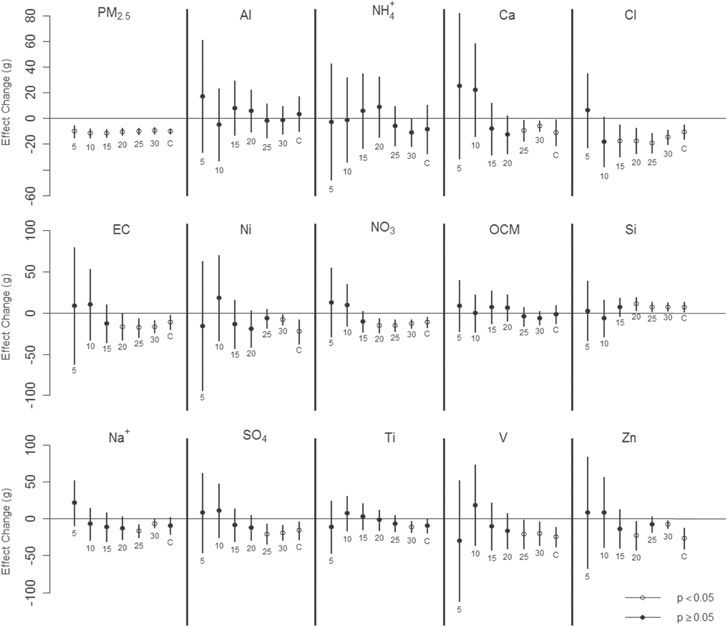
Figure 1. Change in birth weight per IQR increase in PM2.5 total mass and PM2.5 chemical constituents with various buffer sizes. Vertical lines indicate 95% confidence intervals. Below each estimate, the exposure approach is indicated (a number, km, for buffers), C for county-based exposure). IQR values are based on 30 km buffer, and are shown in table 1.
Download figure:
Standard image High-resolution imageOn the other hand, results across buffer sizes were less consistent for most PM2.5 chemical constituents. CIs were generally wider and significant associations were not observed with smaller buffer sizes. County-based exposure assessments were similar to those of larger buffers (20–30 km) (figure 1). For instance, an IQR increase in PM2.5 NO3 was associated with 9.2 g (95% CI: -16.4, 34.7) higher birth weight using a 10 km buffer, but 13.2 g (95% CI: 8.0, 18.4) and 11.3 g (95%CI: 5.1, 17.5) lower birth weight using a 30 km buffer, and county-based exposure, respectively. For PM2.5 Al, NH4+, and OCM, associations were null across all buffer sizes.
Results of logistic regression for LBW are shown in figure 2. Patterns of results across buffer sizes were similar to those of the linear regressions. PM2.5 total mass associations were consistent across all exposure methods, and PM2.5 chemical constituents showed narrower CIs as buffer size increased. While patterns were similar, results for several constituents did not reach statistical significance with larger buffer sizes (e.g. V or Zn).
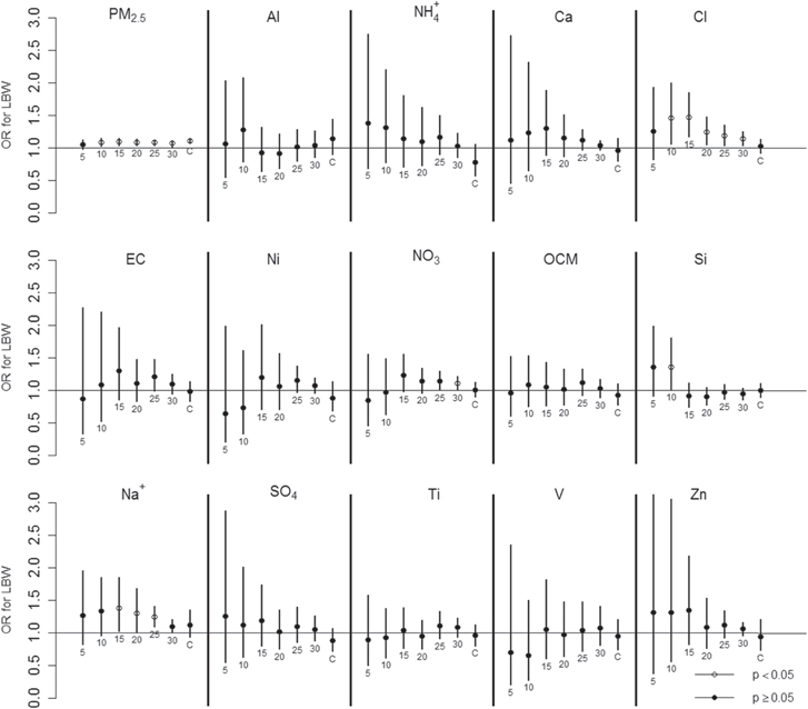
Figure 2. Risk of Odds Ratio for LBW per IQR increase in PM2.5 total mass and PM2.5 chemical constituents with various buffer sizes. Vertical lines indicate 95% confidence intervals. Below each estimate, the exposure approach is indicated (a number, km, for buffers), C for county-based exposure). IQR values are based on 30 km buffer, and are shown in table 1.
Download figure:
Standard image High-resolution imageResults were almost the same using the closest monitor rather than distance weighted average if multiple monitors were available, since monitoring networks of PM2.5 chemical constituents are sparse, resulting in little difference between two assignment methods (supplemental figure 1). Effects of PM2.5 total mass for exposure assigned by the closest monitor are slightly weaker than results using the inverse distance weighted average (supplemental figure 3).
As sensitivity analyses, we implemented two-pollutant linear regression models and trimester exposure models for chemical constituents that showed associations with a 30 km buffer. Supplemental figure 4 showed results of co-pollutant models. For trimester models, pollutants which showed consistent associations in all models were shown (supplemental table 4). Al, Ca, SO4, and V showed associations only at first trimester. Associations were observed in multiple trimesters for PM2.5 total mass and Cl. Si showed lower health risk with higher exposures in the third trimester.
Population characteristics in relation to distance from monitors
As ambient monitors tend to be located in urban areas in the US, mothers living closer to monitors may be in urban environments, lower SES, and more likely to be minority compared to mothers living farther from monitors, which results in different populations and implications for generalizability based on the choice of buffers. We investigated this hypothesis by comparing population characteristics by area based on proximity to monitor: 10 km buffer, area between 10–20 km ring, and 20–30 km ring (table 2). Overall, results indicate that study populations for exposures based on smaller buffer sizes (i.e. mothers living closer to monitors) are more likely to be minority and have lower SES than populations for exposures based on larger buffer sizes (i.e. mothers living farther from monitors). The percent of mothers that were single increased from 21.8% to 38.9% comparing the 10–20 km ring to the 10 km buffer. Percentage of mothers who were young (<25 years old), African American/Hispanic, or had less than high school education was higher for areas closer to monitors. In addition, areas near monitors (10 km buffer) tended to have lower SES neighborhoods compared to areas farther from monitors. The percent of the population in poverty, unemployment rate, and percent with less than high school education are highest within the 10 km buffer. Statistical tests (t-test or chi-square test) showed statistically significant differences between 10 km buffer and 20–30 km ring for all variables in table 2 except infants' gender and maternal alcoholic consumption during pregnancy.
Table 2. Summary of study subject characteristics by area in relation to distance from monitor and county-based assignmentb.
| 0–10 km Buffer (n = 122 585) | 10–20 km Ring (n = 78 801) | 20–30 km Ring (n = 30 537) | County based (n = 221 508) | |
|---|---|---|---|---|
| Birth weight (g) (mean (standard deviation))a | 3411.9 ± 466.2 | 3461 ± 458 | 3476 ± 462 | 3432.7 ± 465.2 |
| Low birth weight (<2500 g)a | 2800 (2.3%) | 1240 (1.6%) | 483 (1.6%) | 4506 (2.0%) |
| Gender | ||||
| Male | 62 447 (50.9%) | 40 081 (50.9%) | 15 533 (50.9%) | 112 895 (51.0%) |
| Female | 60 138 (49.1%) | 38 720 (49.1%) | 15 004 (49.1%) | 108 613 (49.0%) |
| Maternal agea | ||||
| <20 years | 11 131 (9.1%) | 4025 (5.1%) | 1623 (5.3%) | 16 372 (7.4%) |
| 20–24 years | 24 216 (19.8%) | 10 631 (13.5%) | 4225 (13.8%) | 37 769 (17.1%) |
| 25–29 years | 29 762 (24.3%) | 18 541 (23.5%) | 7080 (23.2%) | 52 527 (23.7%) |
| 30–34 years | 34 423 (28.1%) | 26 557 (33.7%) | 10 499 (34.4%) | 67 548 (30.5%) |
| 35–39 years | 18 909 (15.4%) | 15 874 (20.1%) | 5867 (19.2%) | 39 012 (17.6%) |
| ⩾40 years | 4144 (3.4%) | 3173 (4.0%) | 1243 (4.1%) | 8280 (3.7%) |
| Maternal racea | ||||
| White | 60 582 (49.4%) | 60 989 (77.4%) | 25 082 (82.1%) | 135 820 (61.3%) |
| African American | 22 560 (18.4%) | 3633 (4.6%) | 1116 (3.7%) | 27 613 (12.5%) |
| Asian | 6207 (5.1%) | 3472 (4.4%) | 901 (3.0%) | 10 403 (4.7%) |
| Hispanic | 30 678 (25.0%) | 9177 (11.7%) | 2781 (9.1%) | 43 183 (19.5%) |
| Other | 1750 (1.4%) | 979 (1.2%) | 358 (1.2%) | 3007 (1.4%) |
| Unknown | 808 (0.7%) | 551 (0.7%) | 299 (1.0%) | 1482 (0.7%) |
| Maternal educationa | ||||
| Less than high school | 19 858 (16.2%) | 6466 (8.2%) | 2605 (8.5%) | 28 298 (12.8%) |
| High school | 33 955 (27.7%) | 17 804 (22.6%) | 7261 (23.8%) | 56 390 (25.5%) |
| Some college | 25 384 (20.7%) | 17 881 (22.7%) | 6887 (22.6%) | 47 305 (21.4%) |
| College | 41 946 (34.2%) | 36 033 (45.7%) | 13 627 (44.6%) | 87 301 (39.4%) |
| Unknown | 1442 (1.2%) | 617 (0.8%) | 157 (0.5%) | 2214 (1.0%) |
| Maternal marital statusa | ||||
| Married | 74 877 (61.1%) | 61 634 (78.2%) | 23 461 (76.8%) | 151 406 (68.4%) |
| Unmarried | 47 691 (38.9%) | 17 158 (21.8%) | 7071 (23.2%) | 70 076 (31.6%) |
| Unknown | 17 (0.0%) | 9 (0.0%) | 5 (0.0%) | 26 (0.0%) |
| Gestational lengtha | ||||
| 37–38 weeks | 31 168 (25.4%) | 22 012 (27.9%) | 8731 (28.6%) | 60 521 (27.3%) |
| 39–40 weeks | 76 610 (62.5%) | 48 062 (61.0%) | 18 246 (59.8%) | 132 577 (59.9%) |
| 41–42 weeks | 14 807 (12.1%) | 8727 (11.1%) | 3560 (11.7%) | 28 410 (12.8%) |
| Birth ordera | ||||
| First baby | 52 316 (42.7%) | 32 194 (40.9%) | 12 187 (39.9%) | 92 779 (41.9%) |
| Not first baby | 68 962 (56.3%) | 45 952 (58.3%) | 18 122 (59.3%) | 126 538 (57.1%) |
| Unknown | 1307 (1.1%) | 655 (0.8%) | 228 (0.8%) | 2191 (1.0%) |
| Trimester prenatal care begina | ||||
| First trimester | 103 237 (84.2%) | 70 817 (89.9%) | 27 494 (90.0%) | 191 976 (86.7%) |
| Second trimester | 14 977 (12.2%) | 6440 (8.2%) | 2502 (8.2%) | 23 192 (10.5%) |
| Third trimester or later | 2183 (1.8%) | 891 (1.1%) | 359 (1.2%) | 3301 (1.5%) |
| Unknown | 2188 (1.8%) | 653 (0.8%) | 182 (0.6%) | 3039 (1.4%) |
| Alcohol consumption during pregnancy | ||||
| Yes | 536 (0.4%) | 292 (0.4%) | 124 (0.4%) | 934 (0.4%) |
| No | 121 829 (99.4%) | 78 398 (99.5%) | 30 370 (99.5%) | 220 222 (99.4%) |
| Unknown | 220 (0.2%) | 111 (0.1%) | 43 (0.1%) | 352 (0.2%) |
| Tobacco consumption during pregnancya | ||||
| Yes | 6383 (5.2%) | 4944 (6.3%) | 2465 (8.1%) | 12 343 (5.6%) |
| No | 115 804 (94.5%) | 73 704 (93.5%) | 28 011 (91.7%) | 208 584 (94.2%) |
| Unknown | 398 (0.3%) | 153 (0.2%) | 61 (0.2%) | 581 (0.3%) |
| Neighborhood socioeconomic status (mean (%) (standard deviation))c | ||||
| Below poverty levela | 14.6 (13.7) | 7.1 (8.1) | 7.6 (9.0) | 11.5 (12.4) |
| Unemploymenta | 8.5 (6.0) | 5.7 (3.7) | 5.4 (3.5) | 7.3 (5.3) |
| Highest degree is less than high schoola | 17.7 (13.0) | 10.7 (8.7) | 10.5 (8.2) | 14.7 (11.9) |
aVariables show statistically significant difference (p < 0.05) between 10 km buffer and 20–30 km ring. bSubject has at least 37 weeks gestational age (term birth). The number of subjects were determined based on the closest monitor for any pollutant, which has at least one pollutant of gestational exposure for the specified area. cNeighborhood SES is based on residential census tract.
Discussion
We found that PM2.5 total mass is associated with lower birth weight, which is generally consistent with previous research. Similar associations were found in studies conducted in California, eastern US and Europe [11, 39, 40]. A few studies did not find this association [3, 41], which could relate to various chemical structures across the regions [7].
Our findings indicate that effect estimates differ by chemical constituents, implying that the toxicity of PM2.5 might be affected by its chemical constituents. For example, exposure to PM2.5 Ca, Cl, EC, Ni, NO3, Na+, SO4, Ti, V and Zn are associated with lower birth weight with a 30 km buffer, while others constituents are not. These results, however, should be interpreted cautiously; these constituents lost statistically significant associations with other buffers, particularly smaller buffers, and some other constituents exhibited associations at other buffer sizes (figure 1). These findings indicate that different exposure assignment might play a role in the inconsistency of previous studies' results.
Exposure misclassification could contribute to the inconsistency. Some pollutant concentrations can decay over short distances, while others retain the same level for long distances. Supplemental figure 5 shows scatter plots of correlations of monitor pairs and distance between monitors for pollutants within the Northeastern US. For instance, PM2.5 total mass and NO3 show higher homogeneity, while PM2.5 Al and Cl show high heterogeneity within short distances, implying exposure misclassification is more likely for PM2.5 Al and Cl. PM2.5 Al did not exhibit associations with birth weight for any buffer size, which may relate to exposure misclassification even with smaller buffers. Since subject numbers were substantially limited within 5 km from monitors compared to 30 km (table 1), we have limited ability to investigate this issue. Furthermore, exposure to PM2.5 NO3 or Cl was associated with lower birth weight with larger buffers, but smaller buffers produced null results (figure 1). Although association patterns across buffer sizes for NO3 or Cl are similar, Cl exposure estimates likely include higher exposure misclassification than NO3, due to spatial heterogeneity. Our findings suggest that the implications for exposure misclassification due to choice of buffer size differ by pollutant.
Many studies explored PM2.5 total mass and birth weight. For instance, associations are found in Atlanta with 4 mi (6.4 km) buffer and in California with 5 km buffer [1, 8]. Similarly, association between PM2.5 total mass and birth weight is reported in Connecticut with county-based assignment, where the average county area equals that of a circle with 22.6 km radius [28]. These findings are consistent with our results. Limited studies are available for PM2.5 chemical constituents, and identified constituents vary by study. PM2.5 EC and Zn were associated with lower birth weight with 30 km buffer in the current study, which is consistent with a previous study in Connecticut with county-based assignment and a study in California with 20 km buffer [11, 12]. A study in Atlanta found a PM2.5 EC effect with 4 mi buffer [8], while we did not observe associations with small buffers (5–15 km). Likewise, PM2.5 Al NH4+, and Si were associated with birth weight in other research [8, 11, 12], but we did not find associations for Al and NH4+ with any buffers, and found inverse effects for Si with larger buffers. In addition to various exposure assignments among studies, inconsistent results may be explained by correlations among constituents, which differ by region due to local emissions. High correlations are inevitable for PM2.5 constituents, and making interpretation of multi-pollutant models difficult. Adapting source appointment methods could be one way to address this issue [42].
In addition to exposure misclassification from spatial heterogeneity of pollutants, the choice of buffer size has other implications such as sample size. Sample sizes are limited for some pollutants with small buffer sizes, which likely contribute to large confidence intervals (figure 1). Due to fewer monitors, sample sizes are particularly small for PM2.5 chemical constituents with 5 or 10 km buffers, making interpretation of results challenging even though these buffer sizes have less exposure misclassification. Furthermore, areas close to monitors reflect more minority and low SES populations (table 2). Although we and other researchers adjust for demographic and SES variables, the skewed distribution of population characteristics may affect results and comparisons across studies. Figure 3 illustrates that choosing an exposure method involves the tradeoffs of the impacts of exposure misclassification, sample size, and population characteristics. Researchers should take account for those factors when their studies rely on ambient monitors.

Figure 3. Factors affected by buffer size.
Download figure:
Standard image High-resolution image
A key strength of this paper is the use of state-wide detailed birth certificate data for seven years with actual residential location. With this data, we have a long enough time series to avoid cohort bias [43]. In addition, data on the specific residence of each mother enable us to use multiple buffers to assign individual-level exposure and to explore the implications of exposure methods in relation to associations, exposure misclassification, sample size, and population characteristics. Our study adds evidence on associations for PM2.5 and several PM2.5 chemical constituents and birth weight. Our results indicate that some PM2.5 chemical constituents seem more harmful than others, which may indicate that regulating PM2.5 chemical constituents could be more efficient than current regulations based on PM2.5 total mass. Regulating specific PM2.5 chemical constituents might be challenging, because many constituents are highly correlated (supplemental table 1), making difficult to identify single toxic chemical constituent. We tried co-pollutant model for low-correlated constituents, but analysis in more than three pollutants model leads to difficult interpretation. Furthermore, these chemical constituents are likely come from multiple emission sources, which is challenging for regulation [9].
How pollutants affect birth weight is not fully understood from a biological viewpoint, although multiple mechanisms likely occur simultaneously. One potential explanation is that pollutants directly affect fetal growth [14]. Another hypothesis is that some pollutants react with oxygen, affecting blood flow and restraining oxygen and nutrition transfer from mother to fetus [44]. Identification of which constituents and types of particles are most harmful may help inform studies on physiological mechanism.
There are several limitations in this study. First, our exposure estimates rely on ambient monitors. This approach mirrors commonly applied methods in epidemiological studies, but monitor locations tend to be in urban and low SES areas in the US [12, 38]. Therefore exposure values obtained from ambient monitors may not reflect exposure levels of the general population. Additional monitors are needed for sub-urban and rural area, especially for PM2.5 chemical constituents. Utilizing land-use regression, air quality modeling, or satellite imagery to predict concentrations in locations without monitors are emerging approaches. The spatial resolution of satellite methods can reach 1 × 1 km, implying less spatial exposure misclassification [16, 45]. However, these methods have some uncertainties [46], and still require some monitor-based data for inputs and model evaluation [24, 47]. Several papers compared effect estimates based on alternative exposure methods [3, 17–19], but none of them compared effects of PM2.5 chemical constituents. In the future, we could compare effect estimates of chemical constituents based on alternative exposure methods. Another limitation is that we do not have personal time-activity patterns during gestation, describing the locations of mothers (e.g. home, work), which could lead to potential exposure misclassification. Cost and ethics, particularly for vulnerable pregnant women, hinder frequent use of personal monitors over long time periods [48].
Conclusion
In this paper, we explored gestational exposure to PM2.5 and its chemical constituents and birth weight, and the impacts of various buffer sizes to assign exposure. Some PM2.5 chemical constituents appear more harmful than others, and further studies are warranted. To understand toxicity of some PM2.5 chemical constituents, more studies focusing on the relationship between PM2.5 chemical constituents and health are warranted. Improvement of monitoring networks or alternative methods of estimating exposure is desired, since the current situation (e.g. limited monitors, infrequent observation, etc) hinder detailed analysis in epidemiological studies. Homogeneous pollutant levels within a certain distance or geographic unit is a common assumption in many environmental epidemiology studies. Our findings, however, suggest that the validity of this assumption varies by pollutant, and that the choice of exposure method impacts exposure misclassification, sample size, population characteristics, and eventually health associations. This finding should not be interpreted to suggest a particular buffer size, but rather we encourage researchers to consider the related tradeoffs of sample size, exposure misclassification, and demographic characteristics that may affect generalizability to areas outside the buffer. Further studies are warranted in different locations, since the degree of heterogeneity of pollutant levels, monitoring networks, pollutant sources and population characteristics differ by region.
Acknowledgement:
This study was funded by the US Environmental Protection Agency (EPA RD 83479801) and the National Institutes of Health (NIEHS R01ES019560, R01ES016317, R01ES019587). The authors thank Yale Center for Perinatal, Pediatric and Environmental Epidemiology. The authors also appreciate the Connecticut Department of Public Health, Human Investigation Committee, which provided data.
Conflict of interest
none declared.